Lecture 3
Microeconomics Review
August 29, 2025
Demand, Supply, Equilibrium, and Welfare Analysis
Demand and Supply Basics
Demand Curve (Law of Demand):
Quantity demanded decreases as price increases.
\[ Q_d = a - bP, \quad b > 0 \]Supply Curve (Law of Supply):
Quantity supplied increases as price increases.
\[ Q_s = c + dP, \quad d > 0 \]
Marginal Benefit (MB) and Demand — Why Downward?
MB = WTP: The demand curve is a maximum willingness-to-pay curve; it shows the value of the next unit to buyers (their marginal benefit).
Diminishing marginal benefit: Early units satisfy the most valuable uses; later units go to less urgent uses ⇒ MB falls as Q rises ⇒ downward slope.
Purchase rule: Buyers add units while MB ≥ P.
- Aggregating individuals, to sell more units the price must fall to attract buyers with lower WTP ⇒ a downward-sloping demand/MB curve.
Marginal Cost (MC) and Supply
Supply: the set of output levels a firm is willing to produce at each possible market price.
- Selling rule: A firm produces and sells units as long as P ≥ MC.
Supply comes from MC: In perfect competition, firms are price takers. They choose output where P = MC, so the supply curve is the upward-sloping portion of the MC curve (above shutdown).
Why MC rises with output:
- Fixed capacity → adding more output requires using less efficient inputs.
- Overtime, congestion, and rising input costs make each extra unit more costly.
- Fixed capacity → adding more output requires using less efficient inputs.
Economies of scale at low Q: MC may fall initially as fixed costs are spread and efficiency improves. But for supply decisions, only the rising portion of MC matters, since that is where firms operate.
Market Equilibrium
Market clears when:
\[ Q_d = Q_s \]Equilibrium price \(P^{*}\) is such that market clears (\(Q_d = Q_s\)).
Welfare Analysis
Consumer surplus (CS): Area under demand (MB) and above price up to the purchased quantity.
Producer surplus (PS): Area above supply (MC) and below price up to the sold quantity.
Total Surplus (TS) = CS + PS
- TS is the economy’s social welfare measure.
At perfect competitive equilibrium:
- No surplus, no shortage.
- Welfare is maximized–no mutually beneficial trades are left; any quantity above/below \(Q^*\) reduces TS.
- No surplus, no shortage.
Demand, Supply, Equilibrium
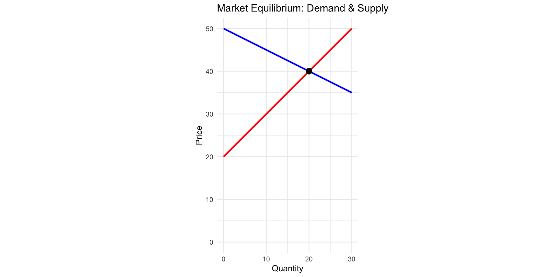
- What are the equations for the demand and supply curves?
Consumer and Producer Surplus
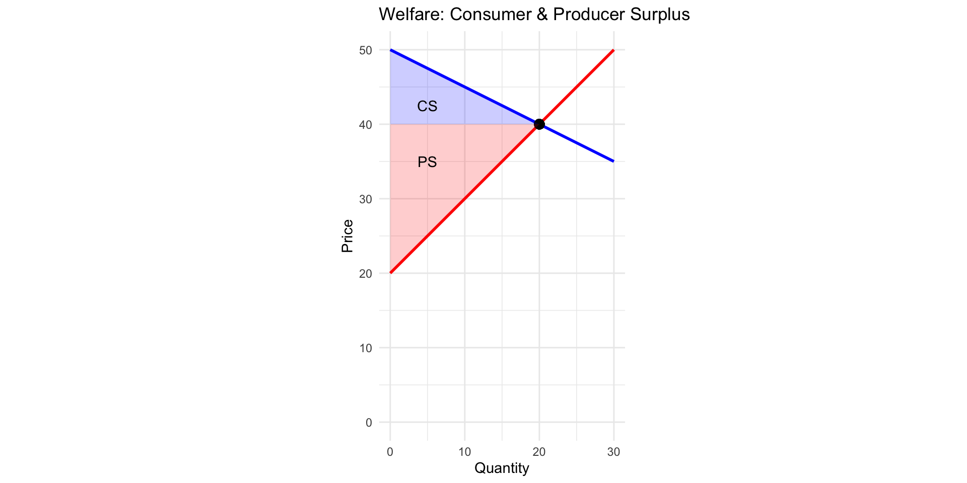
- What are the sizes of CS and PS?
Quantity Regulation (Quota)
Suppose the government sets a quota at
\[ \bar Q = 10 \] so that only 10 units can be traded.At this restricted quantity, suppose that buyers pay MB at \(Q=10\) to sellers.
- How large are consumer surplus (CS) and producer surplus (PS)?
- What is the new total surplus (TS = CS + PS), and how does it compare to the no-quota benchmark?
Tax Example: Setup
- Suppose a per-unit tax t = 5 is imposed on sellers.
- Effect: Supply curve shifts upward by $5.
- How large are consumer surplus (CS) and producer surplus (PS)?
- What is the new total surplus (TS = CS + PS + Tax Revenue), and how does it compare to the no-tax benchmark?
- Reminder: \(\text{Tax Revenue} = t \times Q^{**}\), where \(Q^{**}\) is the quantity traded under the tax.
Deadweight Loss (DWL)
Deadweight loss: the reduction in total surplus that occurs when a market is prevented from reaching the efficient equilibrium quantity.
Interpretation:
- Represents the value of mutually beneficial trades that do not occur.
- Caused by distortions such as taxes, quotas, subsidies, or price controls in a perfectly competitive market.
- Represents the value of mutually beneficial trades that do not occur.
Deadweight loss is the welfare lost to society when output is restricted away from the point where MB equals MC.