| Rate | 0 | 10 | 20 | 30 | 50 | 75 | 100 |
|---|---|---|---|---|---|---|---|
| 1% | 100 | 90.53 | 81.95 | 74.19 | 60.80 | 47.41 | 36.97 |
| 2% | 100 | 82.03 | 67.30 | 55.21 | 37.15 | 22.65 | 13.80 |
| 3% | 100 | 74.41 | 55.37 | 41.20 | 22.81 | 10.89 | 5.20 |
| 4% | 100 | 67.56 | 45.64 | 30.83 | 14.07 | 5.28 | 1.98 |
| 5% | 100 | 61.39 | 37.69 | 23.14 | 8.72 | 2.58 | 0.76 |
| 6% | 100 | 55.84 | 31.18 | 17.41 | 5.43 | 1.26 | 0.29 |
| 7% | 100 | 50.83 | 25.84 | 13.14 | 3.39 | 0.63 | 0.12 |
| 8% | 100 | 46.32 | 21.45 | 9.94 | 2.13 | 0.31 | 0.05 |
| 9% | 100 | 42.24 | 17.84 | 7.54 | 1.34 | 0.16 | 0.02 |
| 10% | 100 | 38.55 | 14.86 | 5.73 | 0.85 | 0.08 | 0.01 |
Lecture 9
Balancing the Present and Future: The Discount Rate
October 24, 2025
The Discount Rate
Why Discount the Future?
- In most environmental policies, costs/benefits often occur at different times
- Converting everything to real (inflation-adjusted) dollars handles inflation—but not time preference
- People (and societies) often prefer benefits now (investment opportunity, uncertainty, impatience)
- Therefore we apply discounting to compare future and present values on a common basis
Note
- Idea: $100 today can be worth the same as $200 ten years from now at an appropriate discount rate.
Present Value (PV) Formula
Let \(X_t\) be a cost/benefit received in \(t\) years and \(r\) the discount rate:
\[ \text{PV}(X_t) \;=\; \frac{X_t}{(1+r)^{\,t}} \]
- Further in time (\(t\uparrow\)) → PV falls
- Higher discount rate (\(r\uparrow\)) → PV falls
Tip
- Examples (for \(X_t = \$100\))
- \(r=3\%, t=10 \Rightarrow \text{PV}=\$74.41\)
- \(r=7\%, t=10 \Rightarrow \text{PV}=\$50.83\)
- \(r=3\%, t=10 \Rightarrow \text{PV}=\$74.41\)
How Fast Does PV Decline?
- High \(r\) greatly devalues distant impacts
- \(r=7\%, t=50\Rightarrow \text{PV}=\$3.39\) for $100
- \(r=10\%, t=50\Rightarrow \text{PV}=\$0.85\)
- \(r=7\%, t=50\Rightarrow \text{PV}=\$3.39\) for $100
- Small changes in \(r\) matter a lot over long horizons
- After 100 years, PV at 1% is about seven times greater than the PV at 3%
PV of $100 by Discount Rates and Years
PV of $500 Billion — Comparing Discount Rates
- Question
- Discount rates play a critical role in evaluating long-term issues such as climate change.
- Suppose a climate policy implemented today will reduce future damages by $500 billion, occurring 50 years from now.
- Two present values of this damage reduction are shown below.
- Which value corresponds to a 2% discount rate, and which corresponds to a 5% discount rate?
- Discount rates play a critical role in evaluating long-term issues such as climate change.
- $185,763,941,063
- $ 43,601,863,486
- 💡 Why it matters: Even small differences in the discount rate can dramatically change how much we value the future — and therefore, how much we act today.
💡 Quick Detour: The Value of Manhattan Island
- The funds used to purchase Manhattan Island for $24 in 1626!
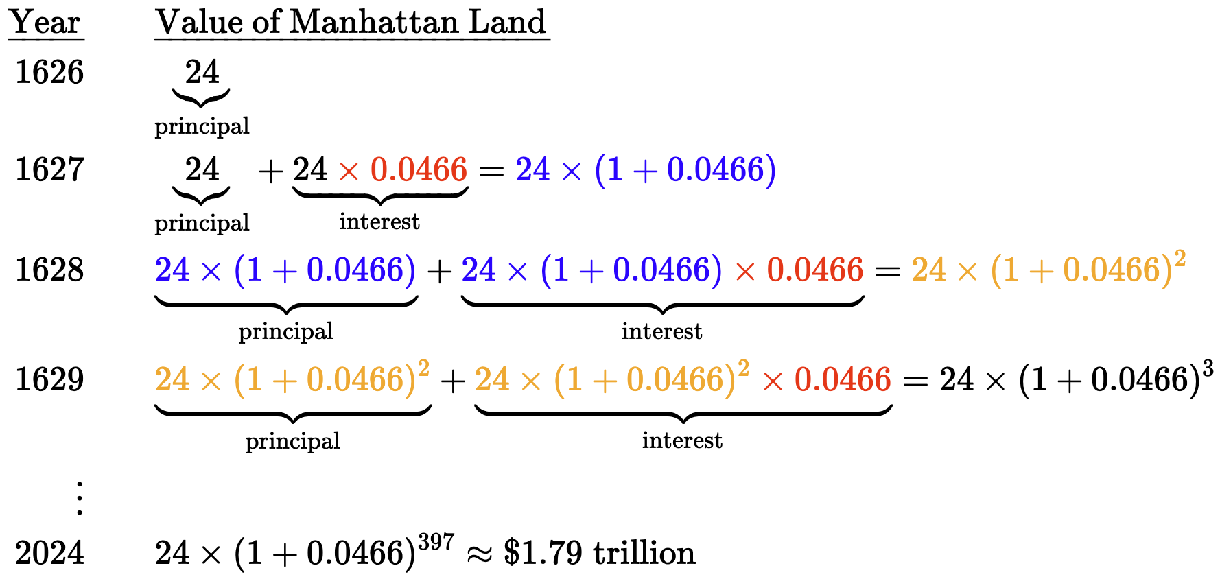
💡 Quick Detour: The Rule of 72
A simple way to estimate how long it takes for a value to double given a fixed annual growth (or interest) rate.
\[ \text{Years to Double} \approx \frac{72}{r} \]
where \(r\) is the annual percentage rate (not in decimal form).
- The higher the rate of return, the faster the doubling.
- Works well for rates between 2% and 15%.
- Useful for understanding economic/financial growth, inflation, or discounting.
- Example: If the economy grows at 3% per year, its size doubles in about 24 years.
Choosing the Discount Rate: Two Approaches
Why Discount the Future?
The discount rate answers a fundamental question:
At what rate should society discount future benefits so that sacrificing one unit of consumption today is fairly balanced by gains to future well-being?
- This rate reflects how we value the future relative to the present, and it can be determined in two main ways:
- Through observed market outcomes → the market-based (descriptive) approach
- Through ethical principles about intergenerational welfare → the social (prescriptive) approach
Linking \(\color{#0072b2}{\eta}\), Diminishing Utility, and Fairness
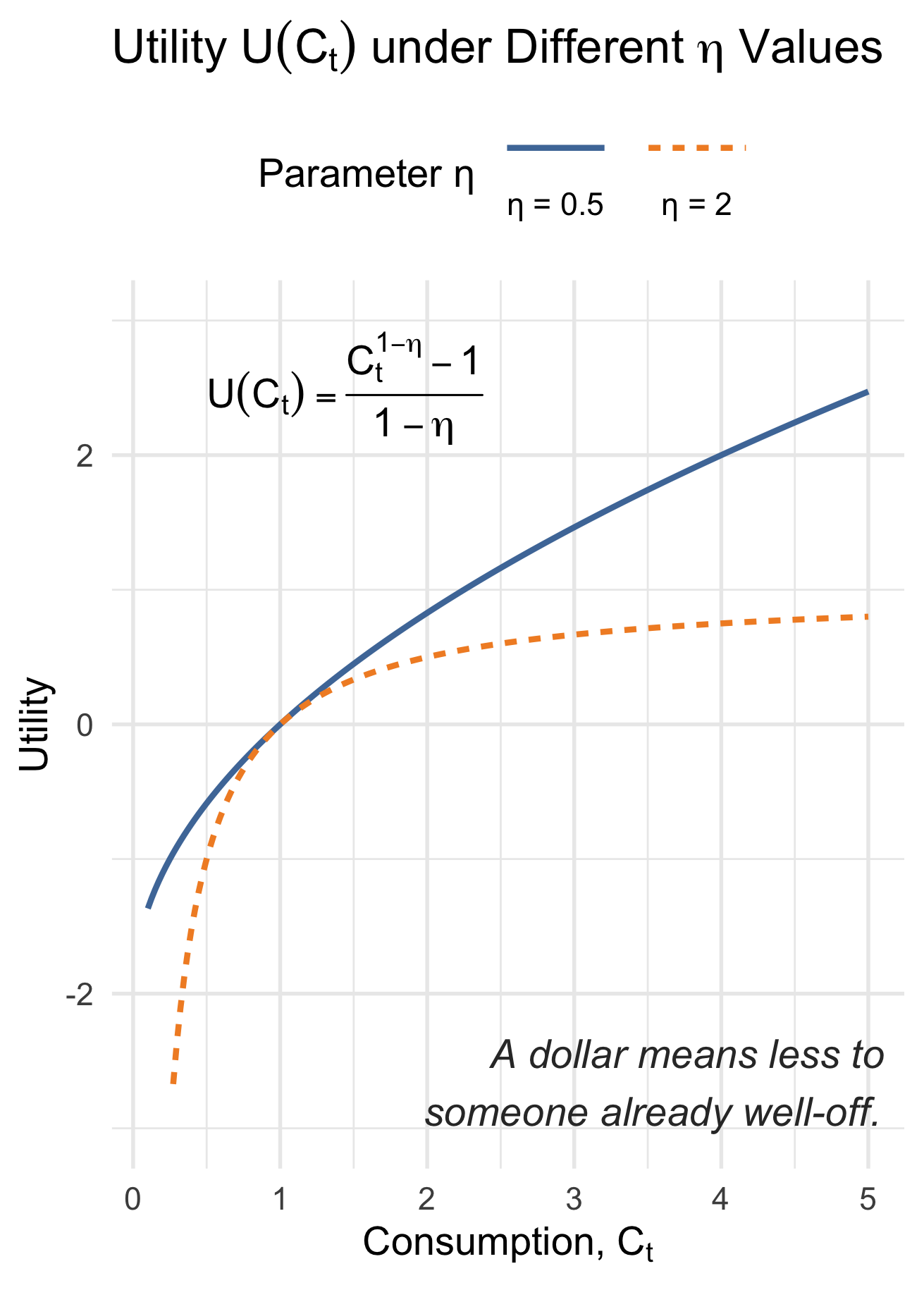
- Higher \(\color{#0072b2}{\eta}\) → Faster Diminishing Marginal Utility
- The extra satisfaction from each additional dollar drops faster as consumption rises.
- Higher \(\color{#0072b2}{\eta}\) → Stronger Concern for Equality
- Because extra consumption benefits the poor more than the rich, a higher \(\color{#0072b2}{\eta}\) means society places greater weight on poorer or earlier generations when choosing how to allocate resources (\(C_{t}\) and \(I_{t}\)) over time.
⚖️ Dynamic Efficiency and Resource Allocation
- Resource Allocation Across Generations: In each period \(t\), total income (\(Y_t\)) can be used for consumption or investment:
- Consumption (\(C_t\)): provides immediate welfare for the current generation
- Investment (\(I_t\)): builds future productive capacity, benefiting future generations
- Consumption (\(C_t\)): provides immediate welfare for the current generation
- To maximize well-being across generations, dynamic efficiency seeks a path that balances present and future welfare:
- How much of today’s output should we consume now versus invest for the future (e.g., in renewable energy or infrastructure)?
- The \(\text{SDR}_{t} = \color{#d55e00}{\rho} + \color{#0072b2}{\eta}\cdot \color{#009e73}{g}_{t}\) provides the answer.
- How much of today’s output should we consume now versus invest for the future (e.g., in renewable energy or infrastructure)?
Discounting Climate Change — Two Lenses
| Feature | Market-based | Ethical |
|---|---|---|
| Approach | How markets actually value the future | How we ought to value the future |
| \(\rho\) | \(1\%\) | \(0.1\%\) |
| \(\color{#0072b2}{\eta}\) | \(1.5\) | \(1.0\) |
| \(\color{#009e73}{g}\) | \(2.25\%\) | \(1.3\%\) |
| Resulting rate | \(\approx 4.4\%\) | \(\approx 1.4\%\) |
| Policy implication | Supports gradual mitigation — high SDR discounts future damages more heavily, making near-term action seem less urgent | Strong case for immediate, large cuts — low SDR gives high present value to avoiding long-term damages |
1️⃣ Market-Based (Descriptive) Approach
Note
The Opportunity Cost of Capital is the return forgone when spending $1 today on a project, instead of investing that same $1 in the best available alternative (for example, in private capital markets or government bonds).
- Set SDR \(\approx\) low-risk market return (e.g., government bonds or average real return on capital)
- Logic: Funds spent today could have been invested — the opportunity cost of capital determines the appropriate SDR
- Idea: Society’s time preference between present and future consumption is revealed through saving, investment, and consumption decisions, as reflected in observed market returns and long-run economic growth.
- Caveat: Market rates change over time
- Very low in the 2020s; very high in the early 1980s
1️⃣ Market-Based (Descriptive) Approach
“What do markets reveal about valuing the future?”
- Sets parameters based on observed market behavior, not ethical judgments
- \(\color{#d55e00}{\rho}\): higher (≈ 1%) — reflects society’s revealed time preference in saving and investment decisions
- \(\color{#0072b2}{\eta}\) (Higher, ≈ 1.5) — means society places greater weight on poorer or earlier generations
- \(\color{#009e73}{g}\): assumes stronger long-run growth (e.g., 2.25%), consistent with historical productivity trends
- \(\color{#d55e00}{\rho}\): higher (≈ 1%) — reflects society’s revealed time preference in saving and investment decisions
- Result: Higher SDR (≈ 4.4%) → less weight on distant future impacts and supports relatively gradual, cost-efficient mitigation of GHG
2️⃣ Ethical (Prescriptive) Approach
“How should markets actually value the future?”
- Parameters are chosen based on ethical reasoning about intergenerational fairness, rather than market behavior
- \(\color{#d55e00}{\rho}\): very low (≈ 0–0.1%) → future welfare is valued almost equally to present welfare
- \(\color{#0072b2}{\eta}\): low (≈ 1) → society gives less additional value to income gains for richer future generations
- \(\color{#009e73}{g}_{t}\): assumes modest long-run growth (≈ 1.3%), which reflects:
- Gradual improvements in living standards without relying on unsustainably rapid innovation or excessive resource use
- \(\color{#d55e00}{\rho}\): very low (≈ 0–0.1%) → future welfare is valued almost equally to present welfare
- Result: Low SDR (≈ 1.4%) → places greater weight on future generations and stronger justification for early climate action
📊 Policy Relevance & Ethics
- 2018 Survey of Economists on the SDR for Intergenerational Global Projects:
- Mean = 2.3%, Median = 2.0%
- 68% of economists recommend a rate between 1–3%
- Trend: Steady shift toward lower SDR since 2001, reflecting greater concern for long-term welfare
- High SDR → prioritizes the present, discounting future impacts heavily
- Low SDR → gives greater weight to future generations
- In environmental cost–benefit analysis (e.g., climate policy):
- Costs occur now, benefits arise later → a lower SDR supports stronger environmental protection
- Costs occur now, benefits arise later → a lower SDR supports stronger environmental protection
- There is no single “correct” rate — analysts should be transparent, justify their assumptions, and test results through sensitivity analysis.
Social Discount Rate (SDR)
\[ \text{SDR}_{t} = \color{#d55e00}{\rho} + \color{#0072b2}{\eta}\cdot \color{#009e73}{g}_{t} \]