Lecture 13

Market for Pollution: Price vs. Quantity Approaches

Byeong-Hak Choe

bchoe@geneseo.edu

SUNY Geneseo

November 7, 2025

Market for Pollution: Price vs. Quantity Approaches

❓ Why Not Just Regulate?

“If the government knows the socially optimal level of pollution, why not just mandate it directly?”

• Regulation (quantity control) has been the traditional approach, since it seems straightforward:
  • 1970s: U.S. limited SO₂ emissions rather than taxing them.
    
  • 1987: Global ban on CFCs to protect the ozone layer instead of taxing them.
• For climate change, however, economists highlight market-based policies that use prices or permits to guide behavior.
  • Carbon taxes (price-based) and cap-and-trade (quantity-based) are the two main policy instruments for reducing GHG emissions.
• Let’s examine when each—price or quantity—is more effective for achieving climate goals.

🌍 Climate Policy Instruments: The Core Idea

Approach	Instrument	Mechanism	Examples
Price-based	Carbon Tax	Sets a price per ton of CO₂; firms reduce emissions until MC = tax.	Sweden CO₂ tax; Canada’s national carbon pricing system
Quantity-based (with flexibility)	Cap-and-Trade	Sets a cap on total emissions; firms trade emission permits until permit price = MC.	European Union Emissions Trading System (EU ETS); California’s Cap-and-Trade Program

Goal: Achieve climate targets at the lowest total social cost.

🔄 From Goods to Pollution Reduction

To compare price and quantity approaches effectively, we must shift focus:

From the market for a product (like automobile)
→ to the market for pollution reduction (like CO₂) itself.

• In basic models, the only way to cut pollution was to reduce output.
  
• In reality, firms can also adopt cleaner technologies:
  • Power plants install CCUS to capture CO₂.
    
  • Cars use catalytic converters to reduce NOₓ emissions.

👉 This shift helps us analyze abatement decisions directly — how firms respond to taxes (prices) or caps (quantities) when multiple reduction options exist.

⚙️ Market for Pollution Reduction: Carbon Market

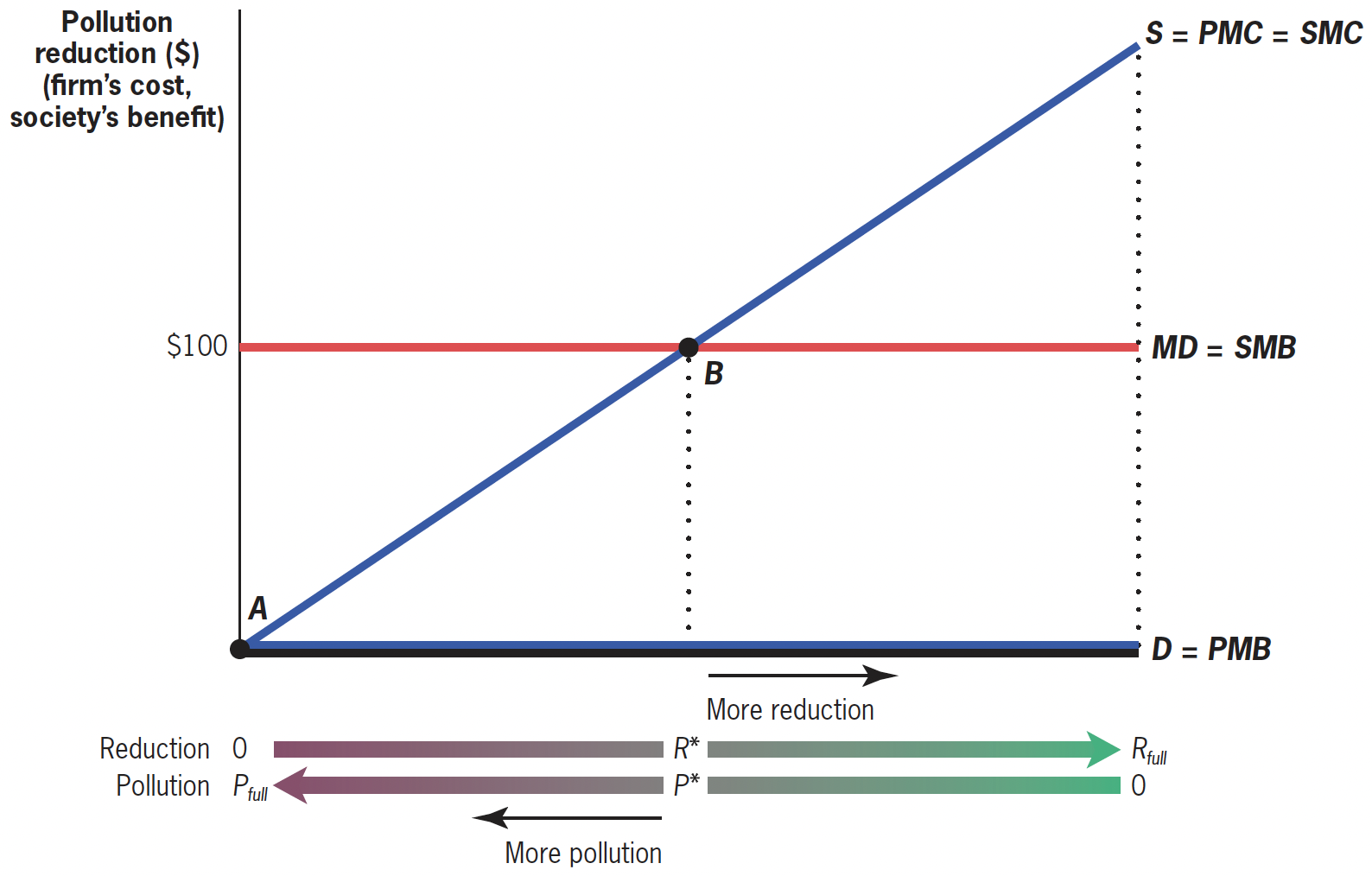
• Marginal Damage (MD) equals SMB — each unit of reduction prevents one unit of harm to society.
  
• Private MC (PMC) equals Social MC (SMC) — there are no externalities in pollution reduction itself.

• \(A\): Free market outcome occurs where PMC = PMB — with no incentive to reduce pollution.
• \(B\): Optimal outcome occurs where SMC = SMB.

💸 Price Regulation: Carbon Tax

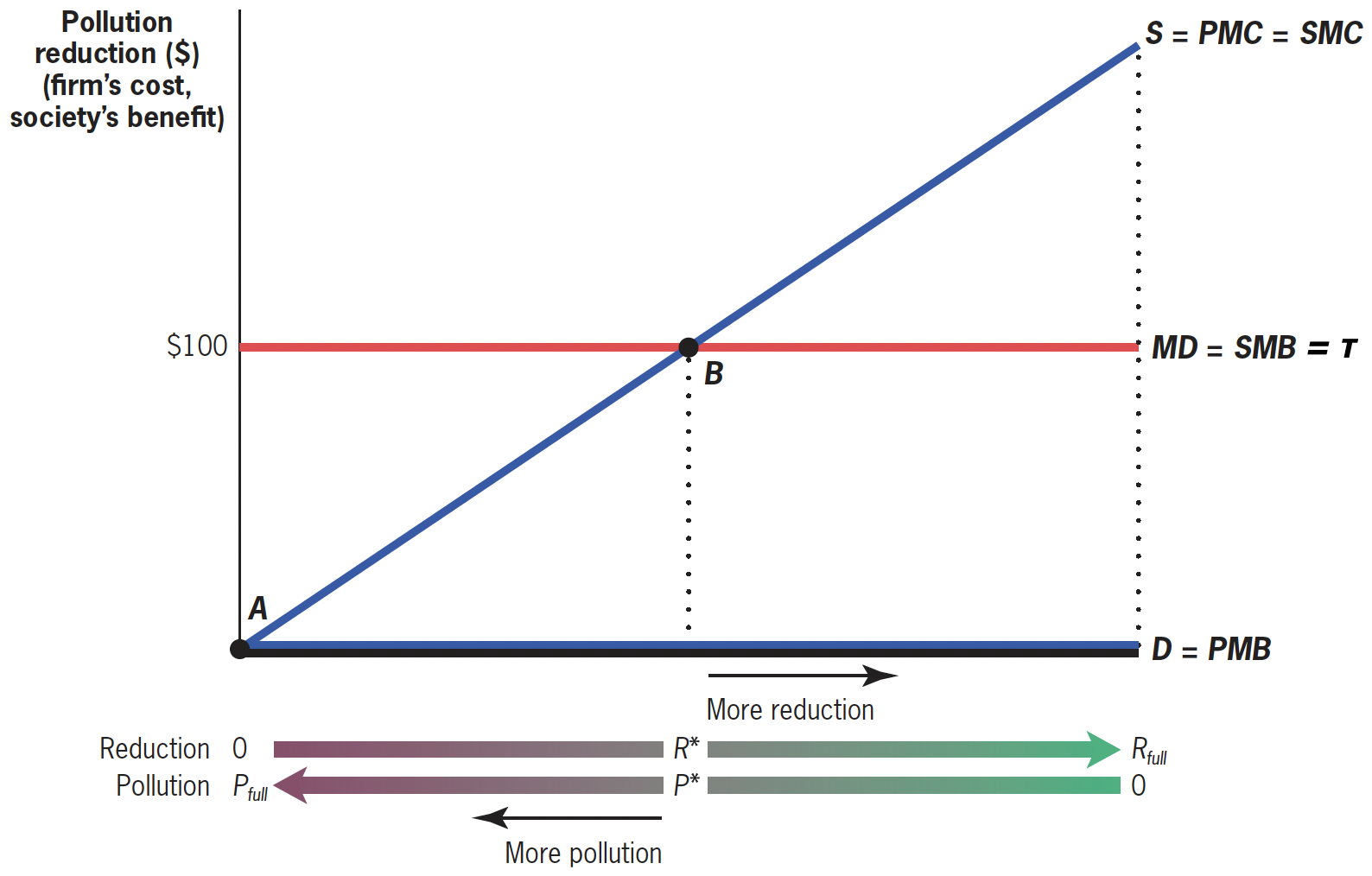
• Government imposes a Pigouvian tax (τ) on each unit of pollution equal to its marginal damage (MD) — for example, $100 per ton of CO₂.

• Each plant reduces emissions as long as its marginal abatement cost (MC) is below τ, and pays the tax on remaining emissions.
  
• Once MC = τ, further abatement would cost more than the tax, so the firm stops reducing.

📏 Quantity Regulation: Mandated Reduction

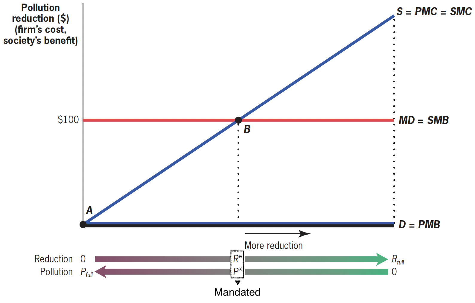
• Regulation: Government simply mandates that firms reduce pollution by the optimal amount (R*).

Note

• If MD is constant, this is manageable; but when MD declines with more reduction, the regulator must know both MD & MC curves to determine either the optimal tax or the optimal quantity.

Heterogeneous Plants

🏭 Heterogeneous Plants

We now consider a case with two plants that have different marginal abatement costs (MC) — a more realistic setting for policy design.

Plant	MC	Efficient Reduction (example)
A (newer tech)	Lower	150
B (older tech)	Higher	50

• In reality, firms differ in technology, age, and fuel mix, leading to unequal costs of pollution reduction.
  
• This setup helps us compare how quantity regulation (like command-and-control) and price-based policies (like a carbon tax & cap-and-trade) perform under realistic conditions.

Note

• Command-and-control regulation: Government mandates specific pollution reductions or sets technology standards that firms must follow directly to control emissions.

🏭 Heterogeneous Plants: Command-and-Control

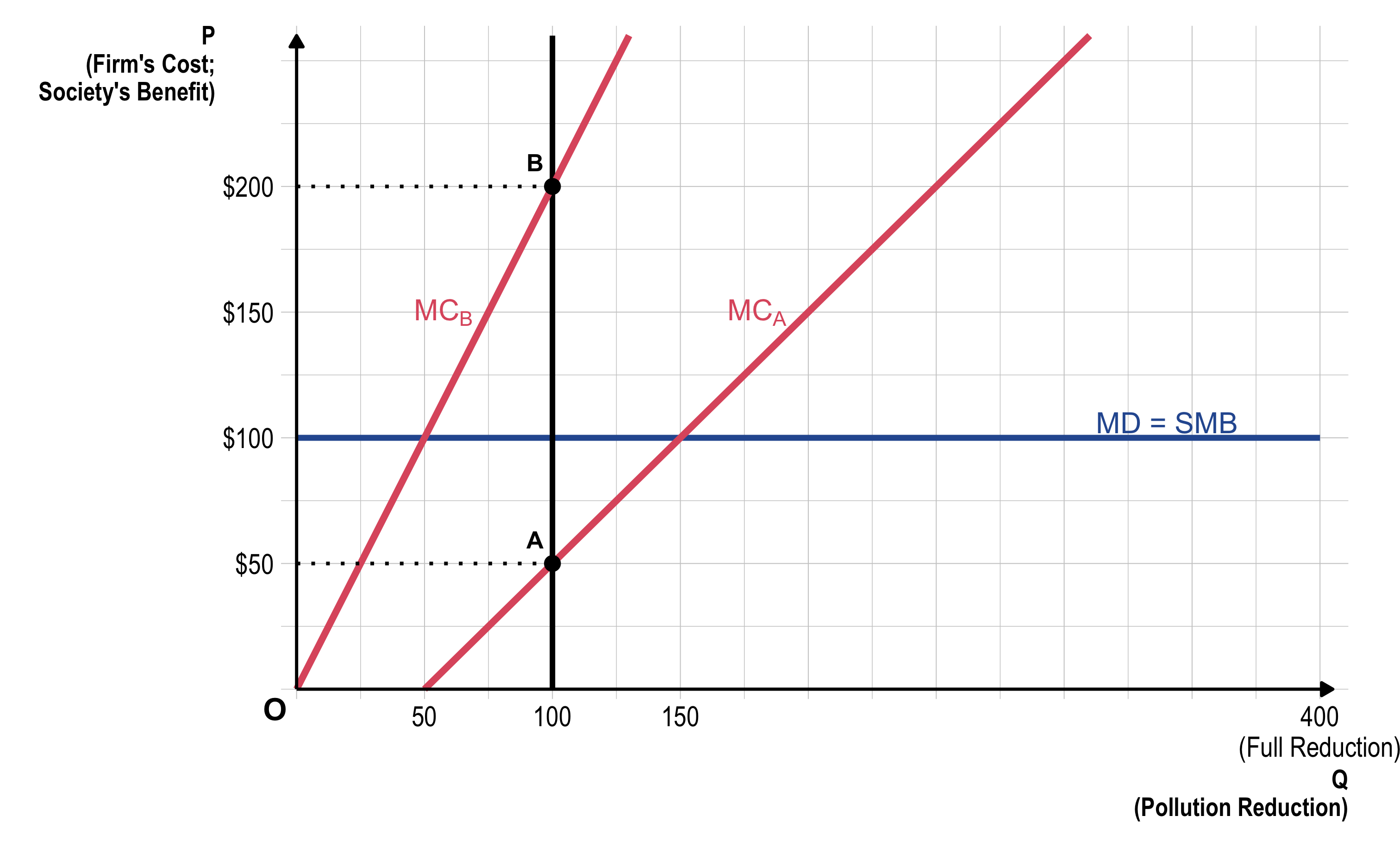
• Equal command-and-control cuts (e.g., 100 units each) simplifies enforcement and compliance — every firm follows the same rule.

• Total Social Cost of Pollution Reduction

\[ \underbrace{\frac{1}{2}\times(100-50)\times50}_{\text{Plant A}} + \underbrace{\frac{1}{2}\times100\times200}_{\text{Plant B}} = \$11,250 \]

🏭 Heterogeneous Plants: Price Regulation

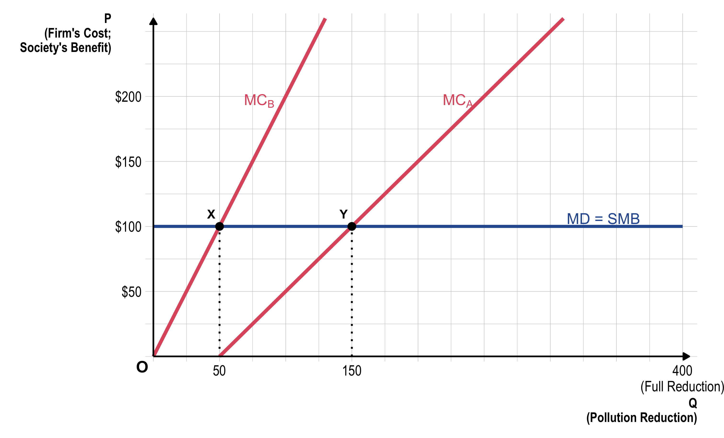
• Under a Pigouvian tax (τ = MD), each firm decides how much to reduce pollution.
  
• Firms abate until their marginal cost (MC) equals the tax rate (τ).

• Total Social Cost of Pollution Reduction

\[ \begin{aligned} \underbrace{\frac{1}{2}\times(150-50)\times100}_{\text{Plant A}} + \underbrace{\frac{1}{2}\times50\times100}_{\text{Plant B}} = \$7,500 \end{aligned} \]

🏭 Heterogeneous Plants: Quantity with Flexibility

• The government sets a total emissions cap (e.g., 200 permits, socially optimal level of pollution) and lets firms trade them.
  • Each permit allows one unit of pollution. (Coase Theorem!)
• A firm will:
  • Abate if its MC is less than the permit price → cheaper to clean than to buy.
    
  • Buy permits if its MC is greater than the permit price → cheaper to pollute than to clean.
    
  • Trading continues until no further mutually beneficial trades exist — just like in a Coase bargain.

MC_A(Q_A) = MC_B(Q_B) = Permit Price.

(Because the cap is the socially optimal level,) Permit Price = MD.\(\qquad\qquad\quad\;\)

• The result: the pollution target is met at the lowest total cost.

–> –> –> –> –>

🏭 Heterogeneous Plants: Summary

Policy Type	What Is Set (Policy Lever)	Who Decides Reduction?	Efficiency
Command-and-control	Set reduction amount (e.g., 100 each)	Government mandates cuts	❌ Inefficient if abatement costs differ
Price Regulation (Tax)	Set price per unit (τ)	Firms choose abatement	✅ Efficient — firms reduce until MC = τ
Cap-and-Trade	Set total emissions cap	Firms trade permits	✅ Efficient — firms trade until MCₐ = MCᵦ = permit price

• ⚖️ Command-and-control regulations are simple but often inefficient.
  
• 💡 Market-based instruments — such as carbon taxes and cap-and-trade — let firms decide how much to abate based on their own costs.
  
• This flexibility ensures the Cost-Effectiveness (Equimarginal) Principle holds: MCs become equalized across firms, leading to an efficient allocation of abatement.
• ✅ Result: the climate target is achieved at the lowest total social cost.

Uncertainty about Costs of Reduction

🌫️ Uncertainty about Costs of Reduction

• In reality, marginal abatement costs (MC) are uncertain — policymakers may not know the exact cost of cutting pollution.
  • They can estimate the overall MC curve, but cannot know its exact slope or position when designing policy.
• This uncertainty means the actual abatement level may differ from what policymakers intended — the socially optimal level.
• The welfare loss from being wrong depends on how sensitive marginal damages (MD) are to changes in emissions.
  
• Under uncertainty, the preferred policy instrument — price (tax) or quantity (cap) — depends on the slope of the MD curve:
  • If MD is steep, errors in abatement lead to large welfare losses.
  • If MD is flat, errors in abatement cause only minor welfare impacts.

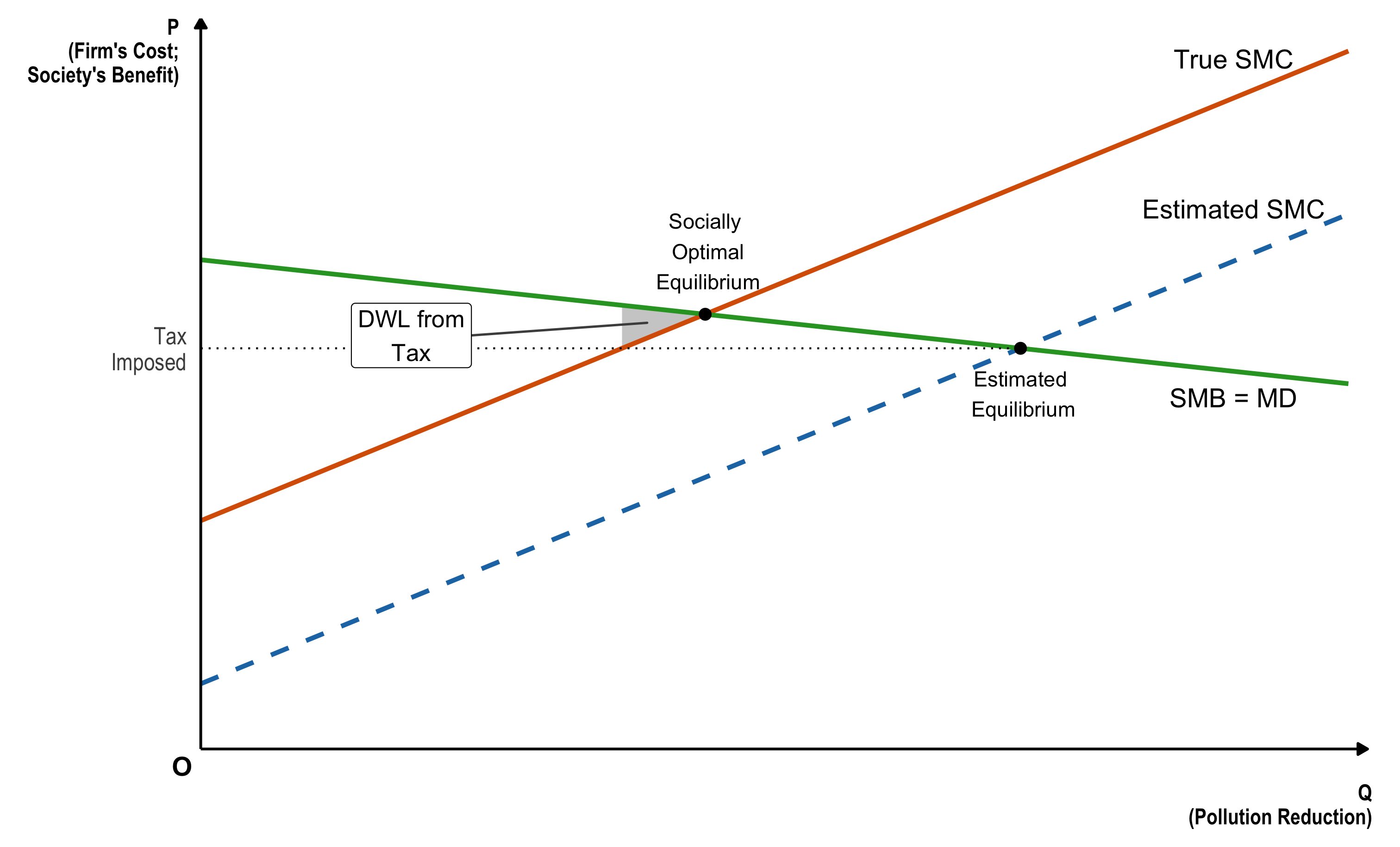
Case 1: Flat Marginal Damage - Tax

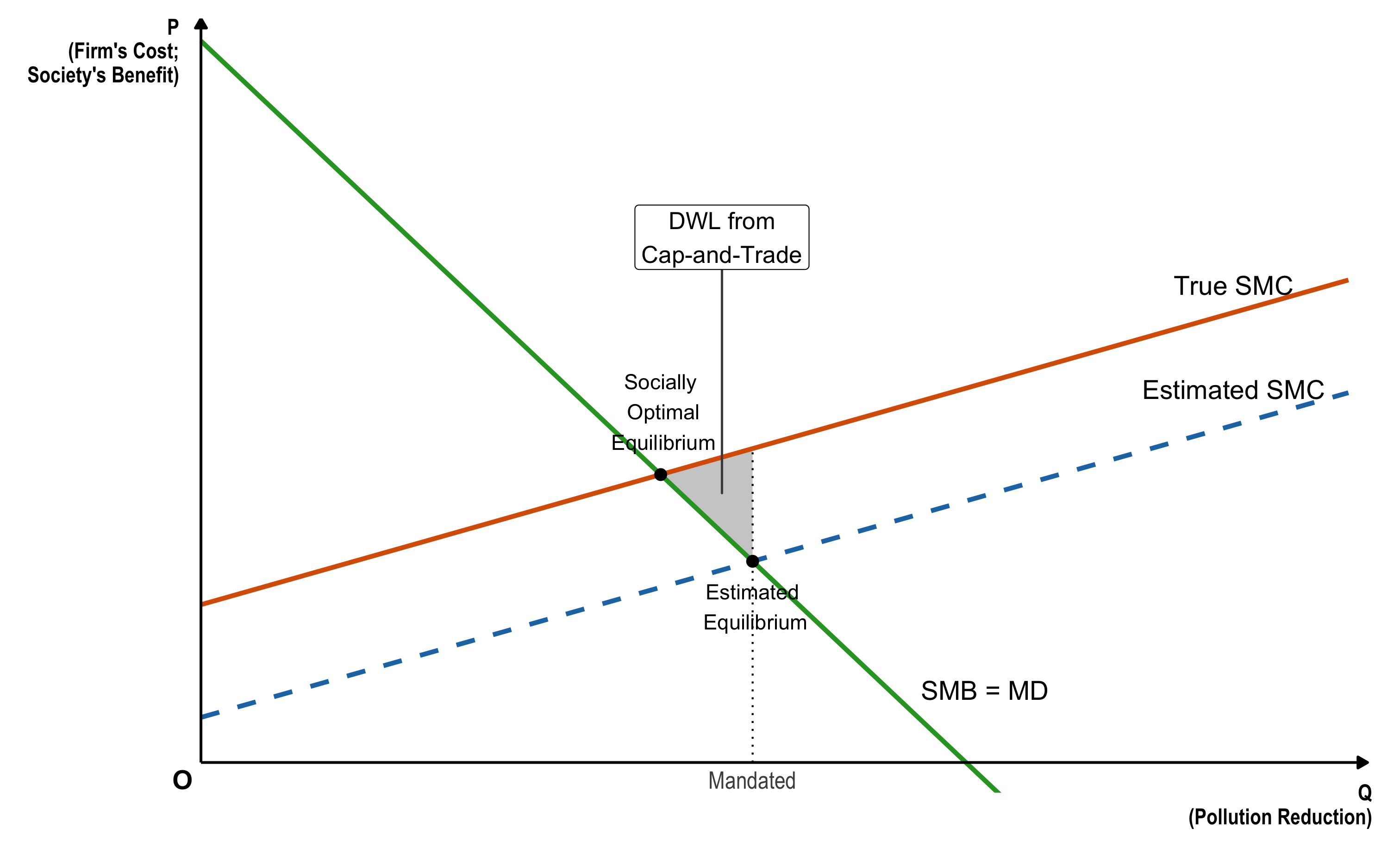
Case 1: Flat Marginal Damage - Cap-and-Trade

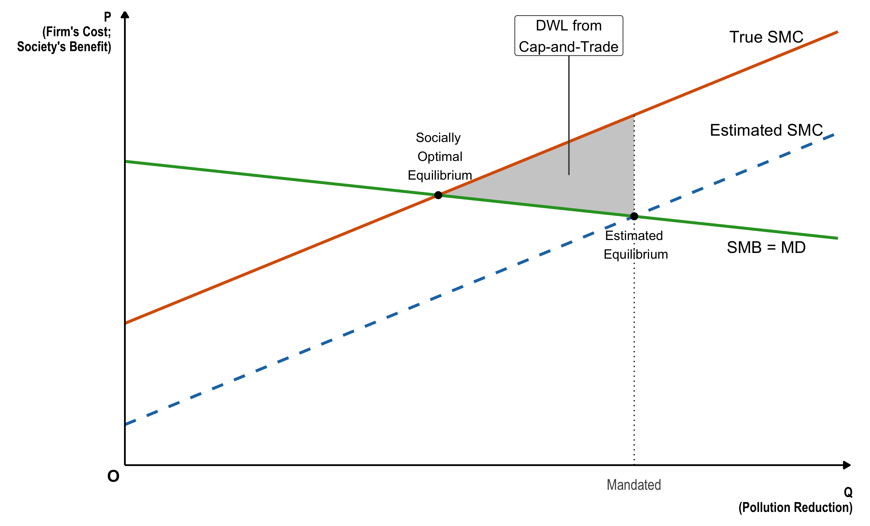
Case 1: Flat Marginal Damage

Tax

Cap-and-Trade

• If the marginal damage (MD) curve is flat (damage changes little with small emission changes)
  → Taxes (price instruments) are preferred.

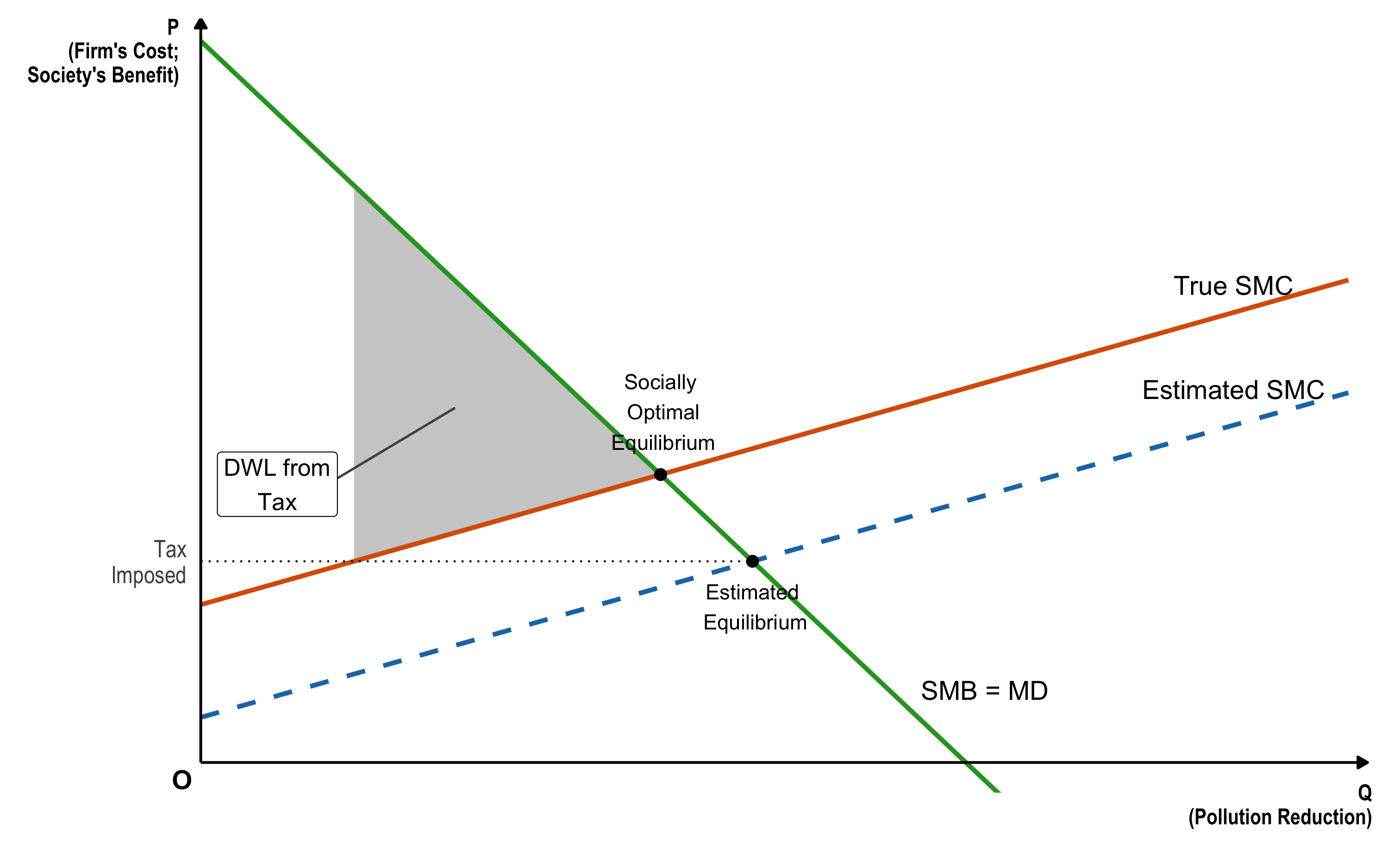
Case 2: Steep Marginal Damage - Tax

Case 2: Steep Marginal Damage - Cap-and-Trade

Case 2: Steep Marginal Damage

Tax

Cap-and-Trade

• If the MD curve is steep (damages rise sharply with small emission increases)
  → Quotas or cap-and-trade (quantity instruments) are preferred.

🌍 Climate Change and Policy Design:

Stock vs. Flow

• Question: Under uncertainty, consider two cases —
  a flat marginal damage (MD) curve vs. a steep MD curve.
  
• 👉 Which case best represents climate change?
  (Hint: the benefits of emission reductions depend on the stock of CO₂, not short-term fluctuations in flow.)

🌍 Climate Change and Policy Design

Carbon Tax vs. Cap-and-Trade

• The benefits of emissions reductions are linked to the stock of greenhouse gases in the atmosphere.
  • What matters for climate damage is the total accumulated CO₂, not short-term fluctuations.
• The costs of emissions reductions are tied to the flow of emissions —
  how much we cut this year or in the near term.

💡 The marginal benefits of emission reductions are insensitive to the current level of abatement
→ small short-run emission changes have little effect on total warming.

• Under uncertainty about abatement costs, a carbon tax is preferred to cap-and-trade for stock pollutants like CO₂ , because emission errors are low-cost, while price errors can be large.

🌍 Carbon Pricing in Practice: Carbon Tax vs. Cap-and-Trade

⚖️ Price vs. Quantity: The Policy Trade-off

• Policymakers face a fundamental trade-off between:
  • Achieving a specific emissions target with certainty, and
    
  • Ensuring stable and predictable costs for firms and consumers.

Carbon Tax

• Provides price certainty — firms know exactly what a ton of CO₂ costs.
• But emissions outcomes can fluctuate with energy demand and economic cycles.

Cap-and-Trade

• Provides environmental certainty — a fixed cap on total emissions.
• But abatement costs can vary widely depending on shocks and economic conditions.

📄 Carbon Tax — Big Advantages

• Simple & Transparent
  • Requires fewer new institutions and less administrative complexity.
• Adapts to Technological Change
  • If abatement costs fall or cleaner technologies become cheaper, a carbon tax leads to greater emissions reductions because firms cut more whenever it becomes cost-effective.
  • Under cap-and-trade, lower abatement costs simply push permit prices downward:
    • Demand for permits falls, but supply is fixed → permit prices drop.
    • Total emissions stay capped, so the overall quantity doesn’t fall—and some firms may even emit more because compliance has become cheaper.

🗺️ Global Map of ETS and Carbon Taxes

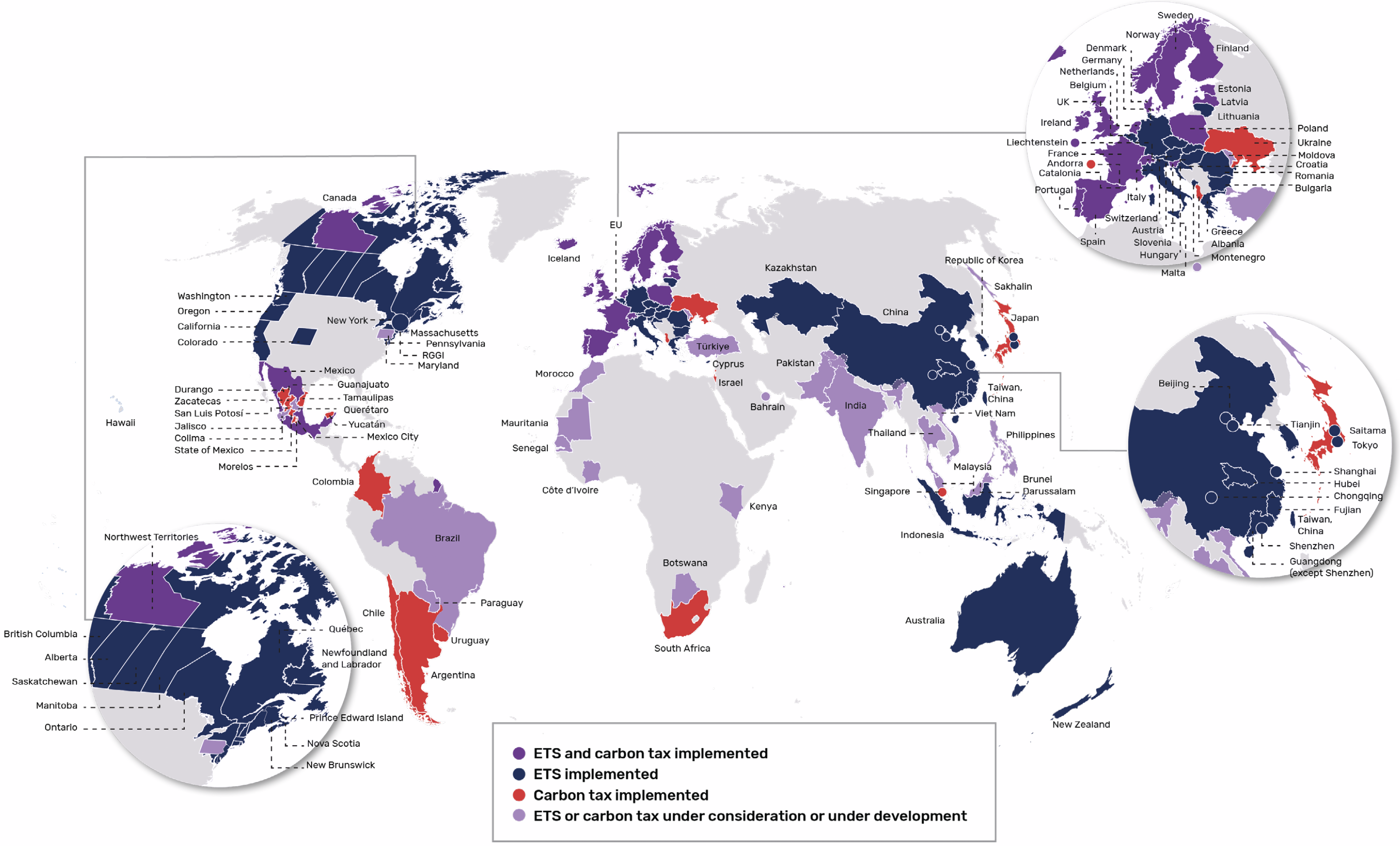
Source: World Bank (2025)

📊 Share of Global GHG Emissions Covered by an Emission Trading System (ETS) or Carbon Tax

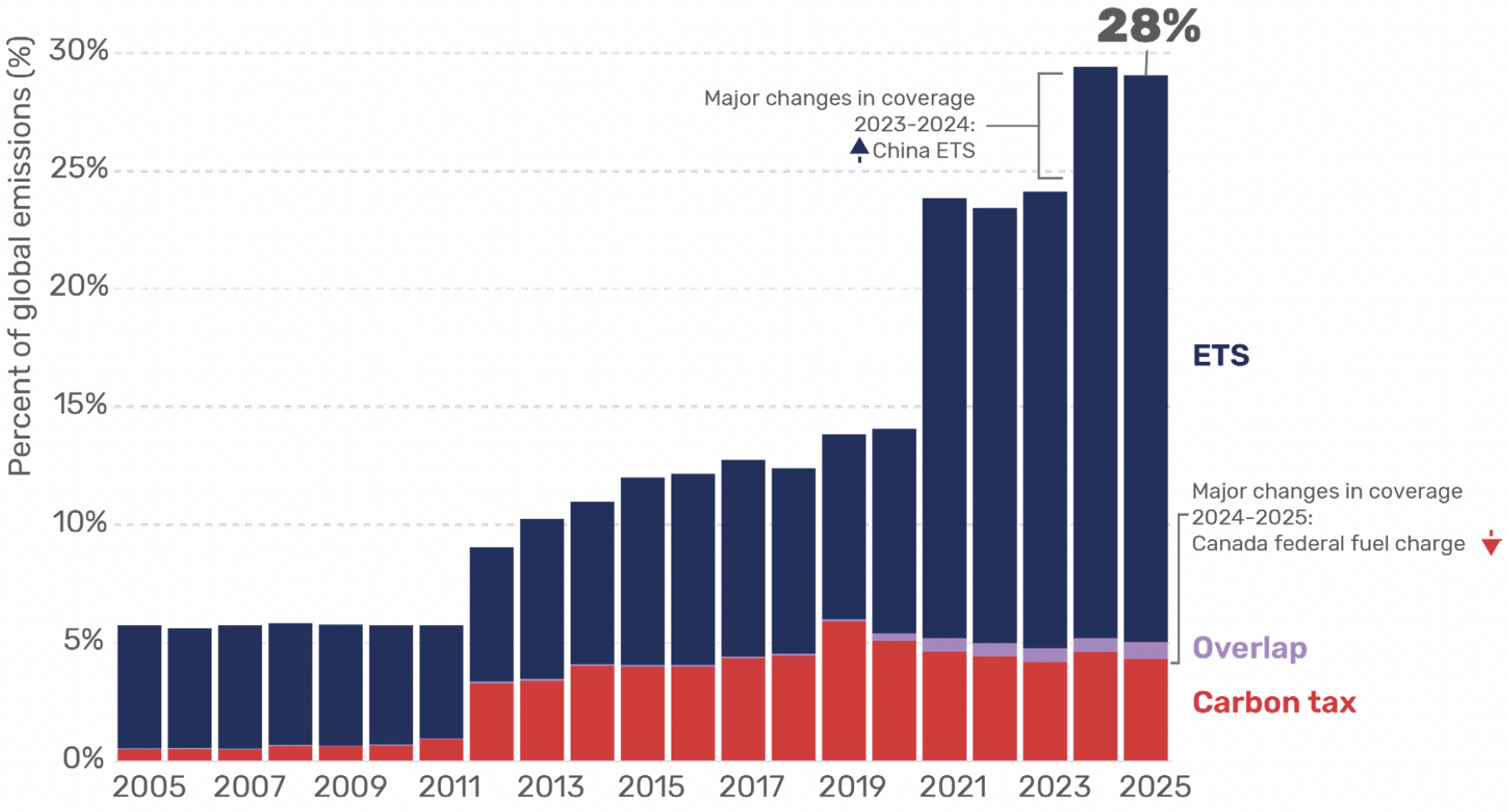
Source: World Bank (2025)

🌍💰️ Emission Coverage and Pricing Level

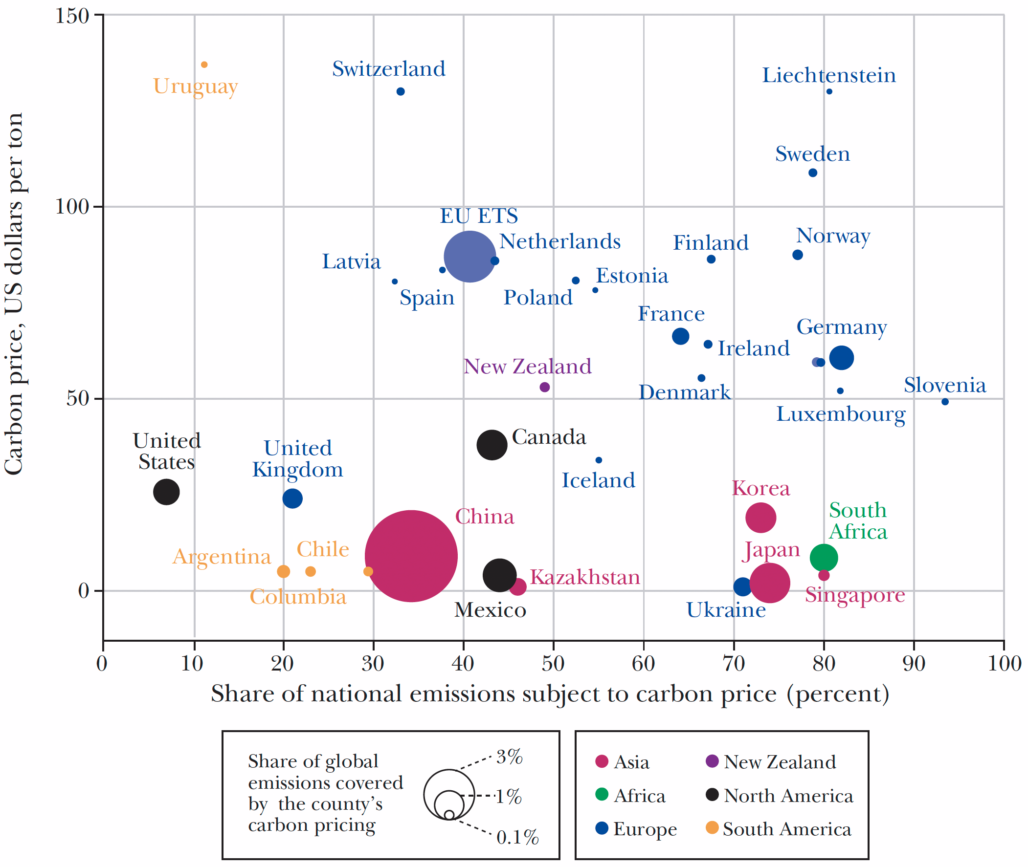
Source: World Bank (2025)

🎯 Why Cap-and-Trade Is More Popular in Practice

“It has become too politically divisive and a distraction from the important issues we are tackling.” Government of British Colombia, “B.C. Eliminates Carbon Tax,” (March 31, 2025)

• Even though economists often prefer carbon taxes (price stability + administrative simplicity), cap-and-trade is more politically feasible:
  • It avoids the politically sensitive term “tax,” reducing public resistance.
    • Introducing a new tax is often politically infeasible, even when it is economically efficient.
  • It enables governments to grant free permits in the early stages, helping secure industry buy-in.
  • It is presented as a flexible, market-driven mechanism, which appeals to policymakers and firms.