Lecture 2

Microeconomics Review for Natural Resource Economics

Byeong-Hak Choe

SUNY Geneseo

August 31, 2026

🧰 Demand, Supply, Equilibrium, and Welfare Analysis

🌲 An Annual Timber Market

  • Buyers: sawmills and wood-products firms use timber to make lumber, paper, furniture, and other products.

  • Sellers: forest owners and logging firms that harvest and deliver timber.

  • \(Q\): truckloads traded per year; \(P\): price per truckload. Assume harvest is sold within the year.

  • Annual demand slopes downward, while annual supply slopes upward: \[ Q_d=a-bP \quad (b>0), \qquad Q_s=c+dP \quad (d>0). \]

  • For the graphs, we use \[ a=100,\ b=2,\ c=-20,\ d=1 \quad\Rightarrow\quad Q_d=100-2P,\ Q_s=-20+P. \]

💵 Demand Shows WTP in This Year’s Market

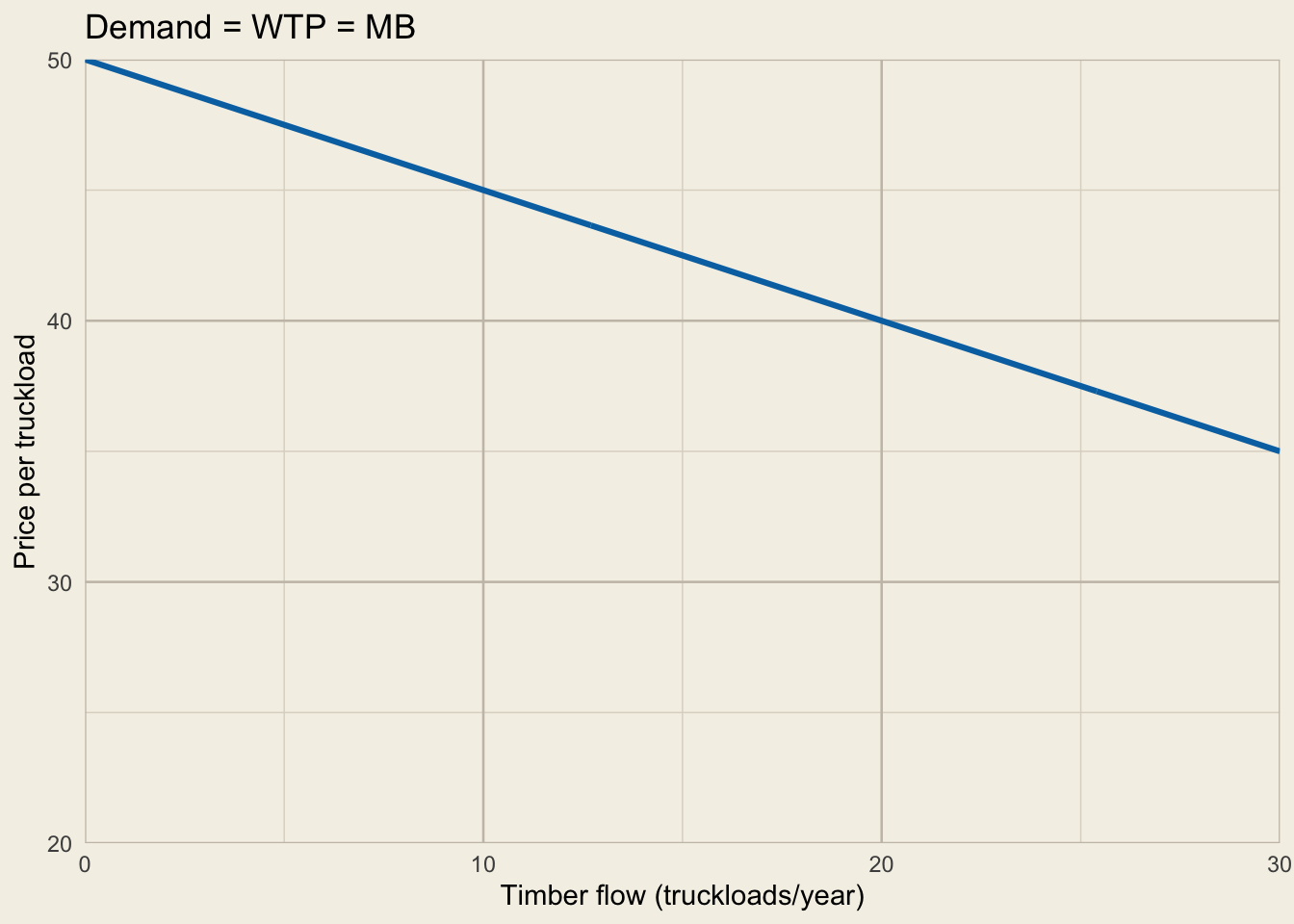
  • Willingness to pay (WTP) is the highest price a buyer would pay for a truckload.

  • WTP for one additional truckload is its marginal benefit (MB). Therefore, the demand curve is also the MB curve.

  • A sawmill’s WTP reflects the value of the lumber and other products it can make from the timber.

  • As annual quantity rises, additional timber goes to lower-value uses, so WTP—and therefore MB—falls.

  • Buyers add truckloads while \(MB \ge P\).

📉 Timber Demand

A downward-sloping annual timber demand curve shows willingness to pay and marginal benefit from zero to 30 truckloads per year.

🏭 Supply Reflects Marginal Cost During the Year

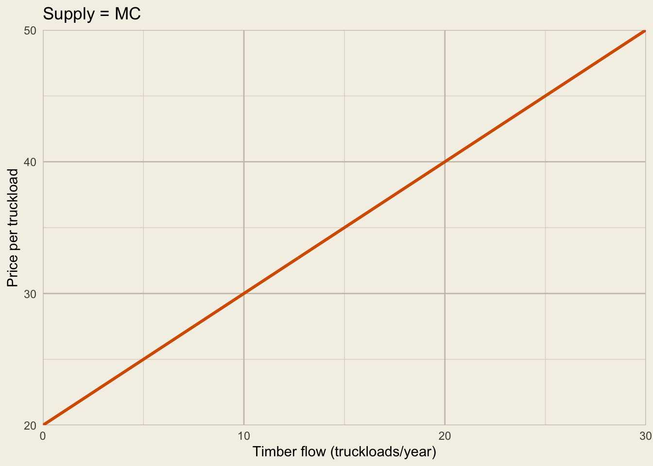
  • Marginal cost (MC) is the added cost of harvesting and delivering an additional truckload during the year.

  • MC rises as annual harvest expands toward higher-cost stands and increasingly constrained crews or equipment.

    • Above the shutdown price, timber sales cover variable operating costs, so harvesting is worthwhile.
    • When \(P>MC\), selling one more truckload adds more revenue than cost, so it increases profit.
    • The firm adds truckloads while \(P>MC\) and stops expanding when \(P=MC\).
    • As price rises, more higher-cost truckloads become worthwhile, so quantity supplied moves up the MC curve.

📈 Timber Supply

An upward-sloping annual timber supply curve shows marginal harvesting cost from zero to 30 truckloads per year.

⚖️ Timber Trade Clears at Equilibrium

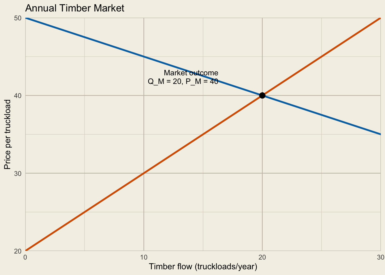
  • At the market price \(P_M=40\), demand equals supply: \[ Q_d = Q_s \]

  • The market quantity is \(Q_M=20\) truckloads per year; there is no shortage or excess supply at \(P_M\).

  • \(Q^*\) denotes the socially optimal quantity. Within this static benchmark, \(Q^*=Q_M=20\); omitted social costs can make them differ.

🎯 Demand, Supply, Equilibrium

Annual timber demand and supply intersect at the private-market outcome Q subscript M equals 20 truckloads and P subscript M equals 40 dollars per truckload.

📊 Surplus Measures This Year’s Gains from Trade

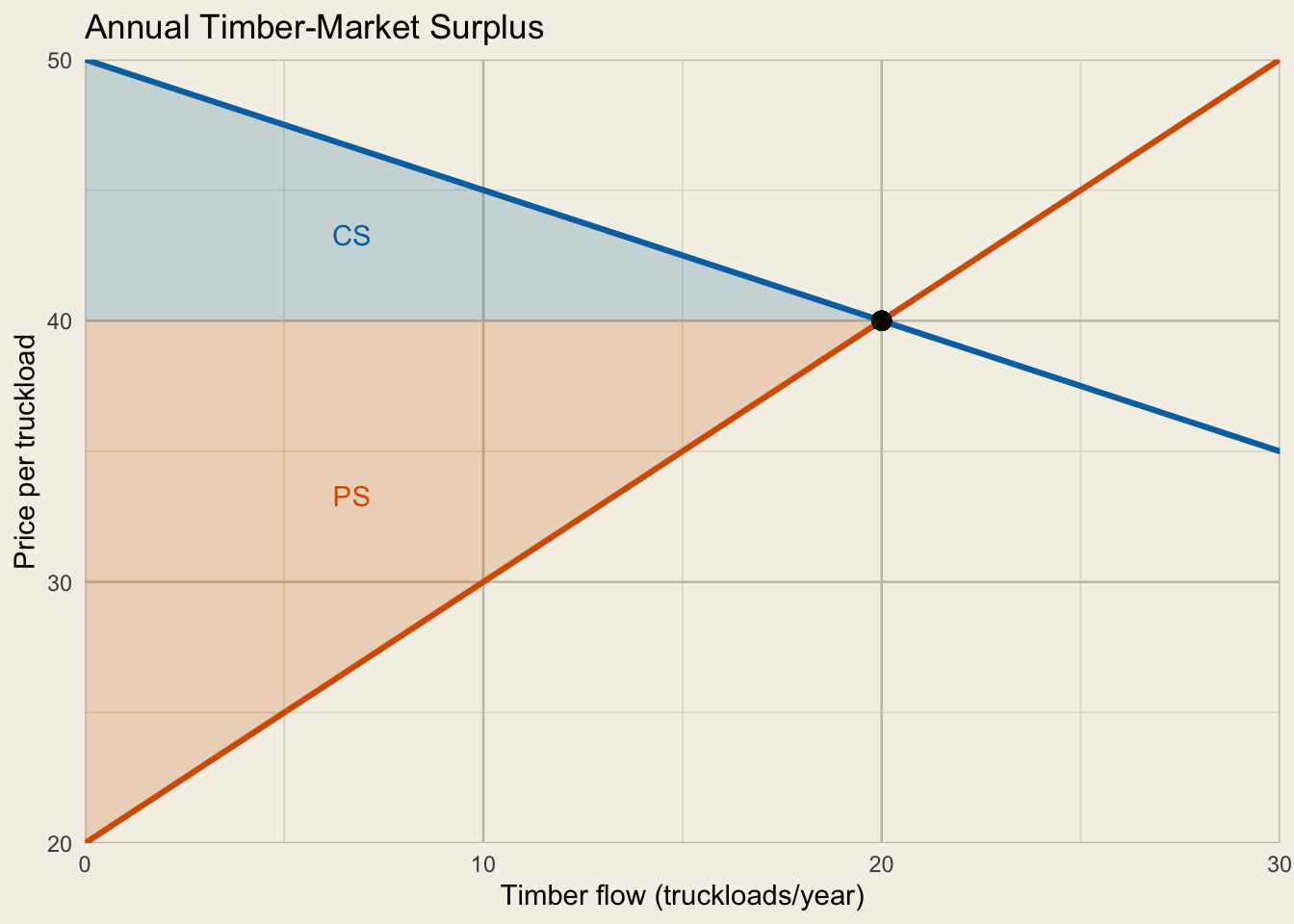
  • Consumer surplus (CS) is buyer surplus: timber buyers’ WTP minus what they pay.

  • Producer surplus (PS) is seller surplus: what timber sellers are paid minus their marginal costs.

  • Total surplus (TS) = CS + PS measures gains from this year’s timber trade.

  • The market outcome \(Q_M\) maximizes this year’s TS only when market MB and MC include all social benefits and costs.

  • The benchmark can fail when:

    • prices omit effects on others (externalities);
    • shared resources allow unrestricted use (open access); or
    • ecosystem services and future scarcity are unpriced.

💰 Consumer and Producer Surplus

The annual timber market at Q subscript M equals 20 and P subscript M equals 40, with consumer surplus shaded above price and producer surplus shaded below price.

  • What are the sizes of CS and PS?

🚧 Quantity Regulation (Quota)

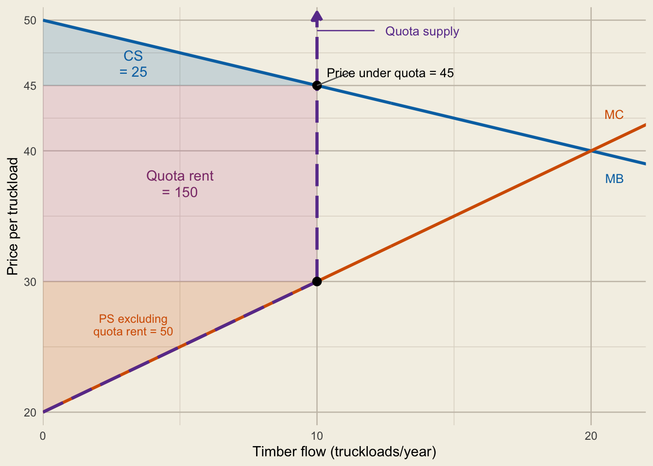
  • Suppose the government limits total timber harvest to 10 truckloads per year.

  • Market supply follows Marginal cost (MC) up to the quota, then becomes vertical.

  • How large are consumer surplus (CS) and producer surplus (PS)?

    • What is the new total surplus (TS), and how does it compare with the no-quota benchmark?

🚧 A Quota Redistributes Surplus

A binding timber quota at 10 truckloads makes effective supply vertical. The graph shades consumer surplus, producer surplus excluding quota rent, and quota rent.

This example has the same surplus outcome as giving timber producers quota permits for free: producers receive the quota rent.

🧾 A Per-Truckload Tax Raises Selling Cost

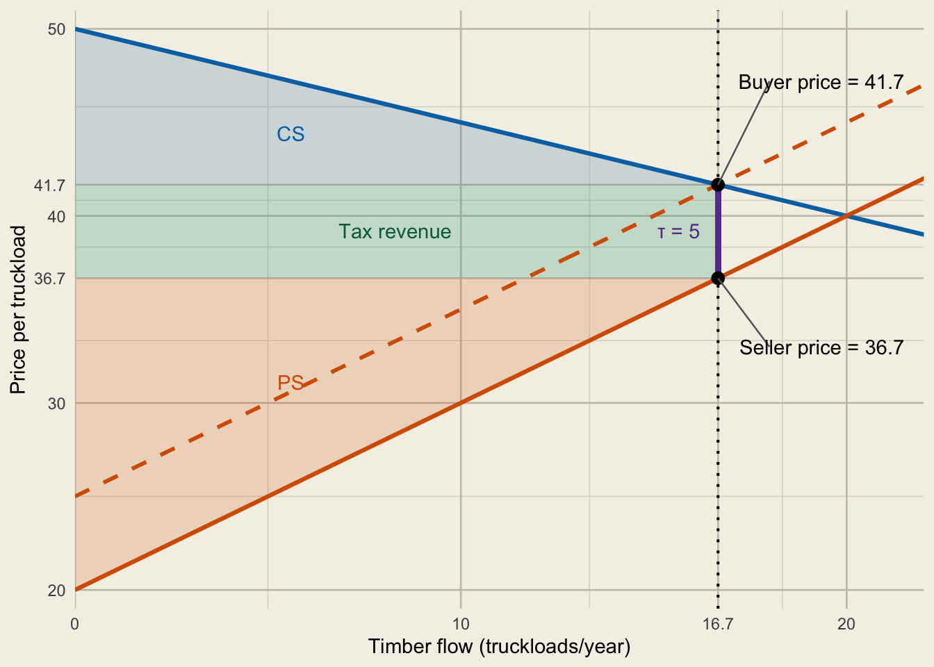
  • Suppose a tax \(\tau=5\) is collected from timber sellers for each truckload sold during the year.

  • In the short run, holding technology and other input costs fixed, the tax does not change technological marginal cost, \(MC(Q)\). It raises the seller’s tax-inclusive marginal cost to \(MC(Q)+\tau\).

  • Sellers need to keep \(P_s=MC(Q)\) on the marginal truckload, so buyers must pay \[ P_b=P_s+\tau=MC(Q)+5. \] Thus, supply plotted against the buyer price shifts upward by \(5\).

  • The tax wedge is \(P_b-P_s=\tau\), and tax revenue is \(\tau Q_{\tau}\). Use the shifted supply curve to find the new quantity, prices, and surplus.

🧾 A Tax Creates a Price Wedge

A per-truckload tax creates a five-dollar wedge between the buyer price and seller price at the tax quantity Q subscript tau of about 16.7, below the market quantity Q subscript M of 20.

  • The per-truckload tax reduces annual timber trade from \(Q_M=20\) to \(Q_{\tau}\approx16.7\) and separates the buyer and seller prices by \(5\).

🔺 Deadweight Loss (DWL)

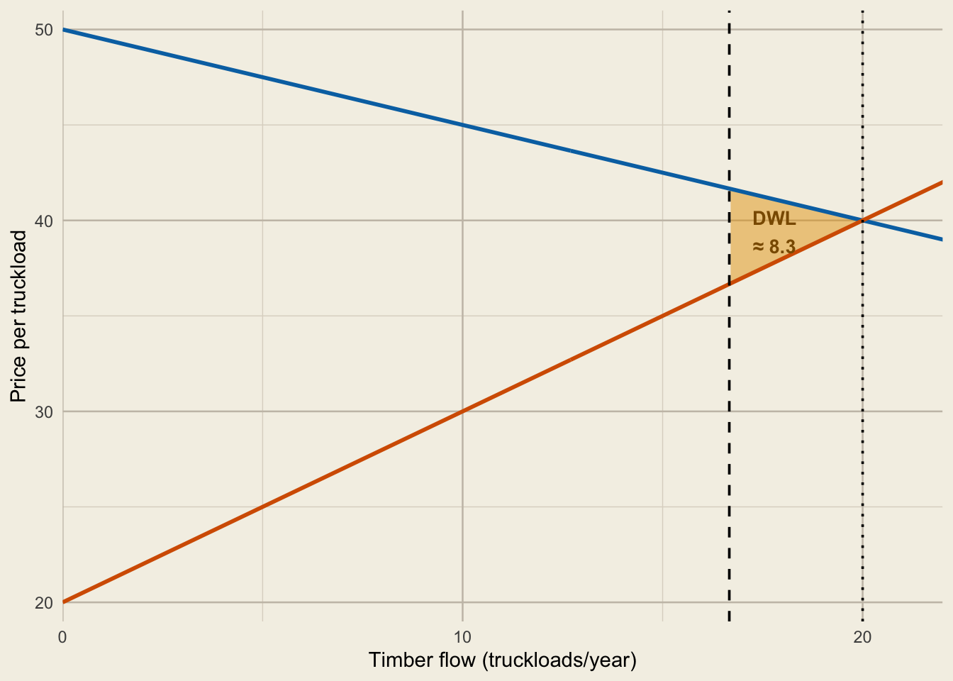
  • Deadweight loss: the reduction in total surplus that occurs when quantity differs from the socially optimal quantity, \(Q^*\).

  • Interpretation:

    • Represents the value of mutually beneficial trades that do not occur.
    • Caused by distortions such as taxes, quotas, subsidies, or price controls in a perfectly competitive market.
  • Deadweight loss is the welfare lost to society when output is restricted away from the point where MB equals MC.

🔺 DWL Is the Value of Missing Trades

Quota: \(\bar Q=10\)
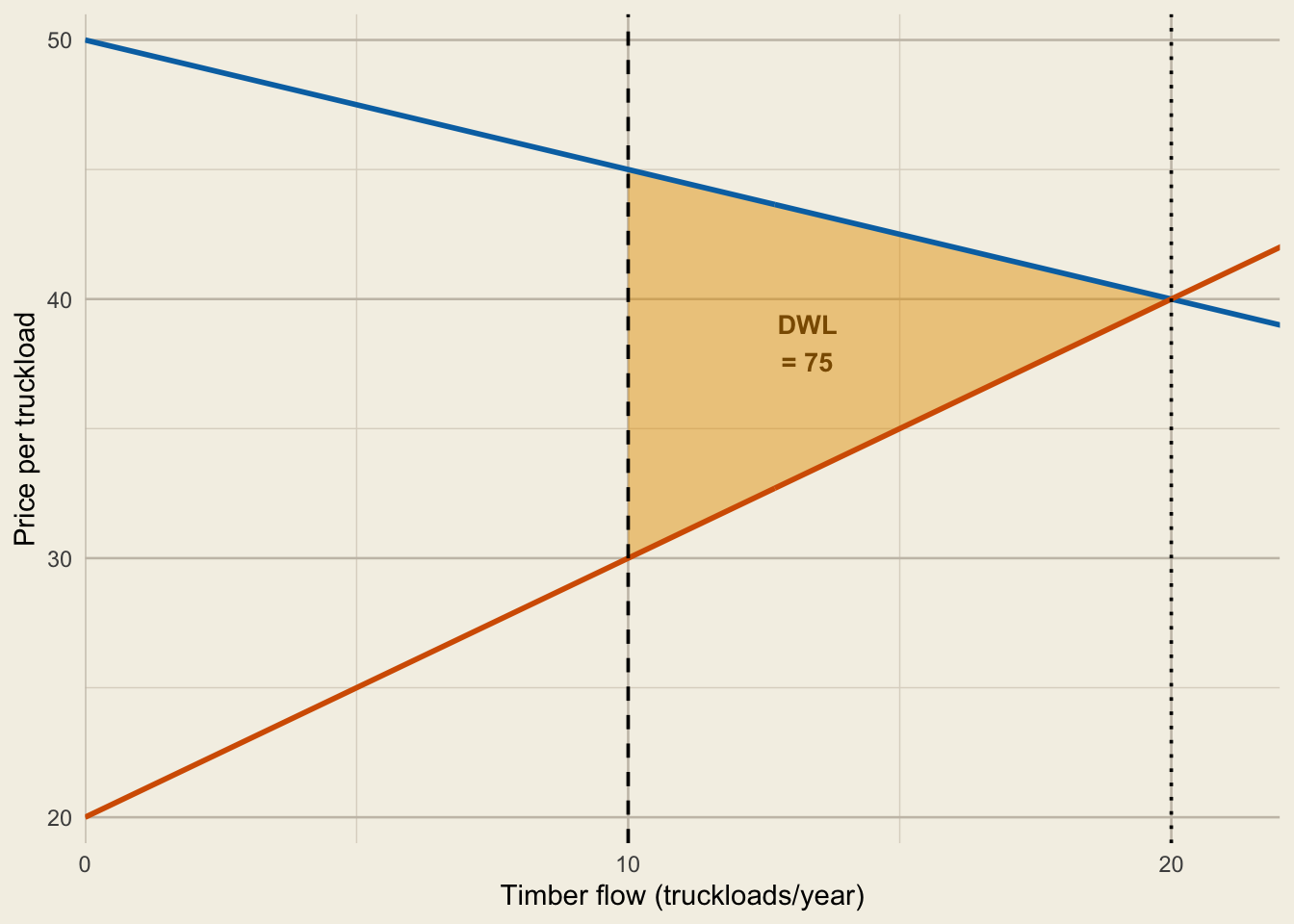
A quota at 10 truckloads creates deadweight loss between the quota quantity and the benchmark social optimum, which equals the market quantity of 20.

Tax: \(\tau=5\)

A five-dollar tax creates deadweight loss between Q subscript tau of about 16.7 and the benchmark social optimum, which equals the market quantity of 20.

  • The orange areas measure annual timber trades for which \(MB>MC\) but the policy prevents exchange.

🌲 Scarcity and Competing Uses

  • The annual timber market can clear at \(Q_d=Q_s\): there is no shortage during the year.

  • Yet the forest has a limited stock of mature trees.

  • Harvesting a tree this year means that same tree is no longer available to harvest in a future year.

  • The value of leaving it available for a future year is an opportunity cost of harvesting it now.

    • Opportunity cost: the value of the best alternative given up when a choice is made.
  • To track that trade-off, we should distinguish the resource stock from the harvest flow.

⏳ This Year’s Harvest Changes Next Year’s Stock

  • Time subscripts: let \(t\) be 2025, so \(t+1\) is 2026.

  • \(S_t\): start-of-2025 stock; \(H_t\): harvest during 2025. If the harvest is sold that year, \(Q_t=H_t\).

  • \(G_t\) is net biological growth (about zero for oil or minerals).

    • For timber: growth of surviving trees plus trees entering the measured inventory, minus natural mortality.

\[ S_{t+1}=S_t+G_t-H_t \]
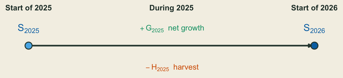
A timeline runs from the start of 2025, with stock S subscript 2025, to the start of 2026, with stock S subscript 2026. During 2025, net biological growth G subscript 2025 adds to the stock and harvest H subscript 2025 subtracts from it.

🧩 What Does Market Clearing Tell Us?

  • If a market clears—if quantity demanded equals quantity supplied—can the natural resource still be scarce?
    • How is scarcity different from a shortage?
    • What is the opportunity cost of harvesting one more tree this year?
  • If the market clears today, does that guarantee that the resource will remain available in the future?
    • What must we know about the forest’s stock, net growth, and harvest?
    • How could a quota or tax affect the stock carried into next year?