Lecture 4

Property Rights, Open Access, and Resource Institutions

Byeong-Hak Choe

bchoe@geneseo.edu

SUNY Geneseo

September 11, 2026

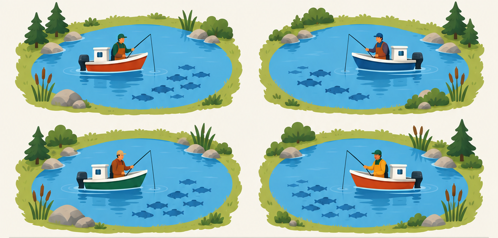
🎣 Classwork 3: Five Fishing Setups

Five fishing setups, two years each, ten choices

🪪 Your Boat and the Ten-Choice Sequence

Bring one internet-connected device.
Use your assigned boat code (A01–A32), not your name.
Use the same fishing-group number and group size for all ten choices.
Each group has 3–5 boats. The lowest-numbered boat present is the stock keeper.

Setup	Fishing setup	Years
1	Your Own Pond	1 and 2
2	Shared Bay: No Catch Limit	1 and 2
3	Group Limit, No Checks	1 and 2
4	Group Limit, Random Checks	1 and 2
5	Limit Enforced at the Dock	1 and 2

The instructor resets the fish to their original level before each new setup.

🐟 Rules Used Every Year

The fish stock

Every setup starts with 9 fish per boat.
- 3 boats: 27 fish
- 4 boats: 36 fish
- 5 boats: 45 fish
Before each year’s catch, nature adds 2 fish per boat.

For shared water,

\[ F_{t+1}=F_t+2n-H_t. \]

Your decision

Choose a catch from 0 through 5 fish.
Choose privately while everyone plays the same setup and year.
Do not discuss catches while a yearly choice is open.
Before Setup 3, your group has 90 seconds to choose a maximum of 1, 2, or 3 fish per boat.
The same group maximum applies in Setups 3–5; a tie or no decision means 2 fish.
Enter only catch; the page calculates the stock.
After Year 2, each fish left is worth 4 future-season points, allocated according to the setup.

💵 Your Group’s Dock Price

If $H$ is group catch and $n$ is the number of boats,

\[ p=10-\frac{H}{n}=10-\text{average catch}. \]

More average catch means a lower dock price.
Each fishing group is a local market; groups with the same average catch receive the same price.
The price is revealed only after every boat in the group submits.

Average catch	Price per fish
0	10
1	9
2	8
3	7
4	6
5	5

📊 Your Catch Points

Your catch $h_i$	Catch cost $C(h_i)$
0	0
1	1
2	3
3	6
4	10
5	15

For your catch $h_i$,

\[ \text{catch points}=h_i \times p- C(h_i). \]

The next fish is increasingly costly to catch.
$p$ is the dock price determined by your group’s average catch.
Catch points measure this year’s revenue minus your catch cost.

🧮 One Unpaid Example

Practice only. Do not submit: four imaginary boats choose catches of 1, 3, 3, and 5 fish.

Group catch: $H=1+3+3+5=12$ fish.
Average catch: $H/n=12/4=3$ fish per boat.
Dock price: $p=10-3=7$ points per fish.
A boat catching 3: $3(7)-6=15$ catch points.
Fish next year: $36+2(4)-12=32$ fish.

Before the real game begins, the fish return to the setup’s original level.

🏞️ Fishing Setup 1: Your Own Pond

Four boats, each fishing in a separate pond.

You manage a separate pond that starts with 9 fish.
Only your catch changes your pond.
Nature adds 2 fish before each year’s catch.

\[ f_{i,t+1}=f_{i,t}+2-h_{i,t}. \]

After Year 2, each fish left is worth 4 points to you.

🌊 Fishing Setup 2: Shared Bay, No Catch Limit

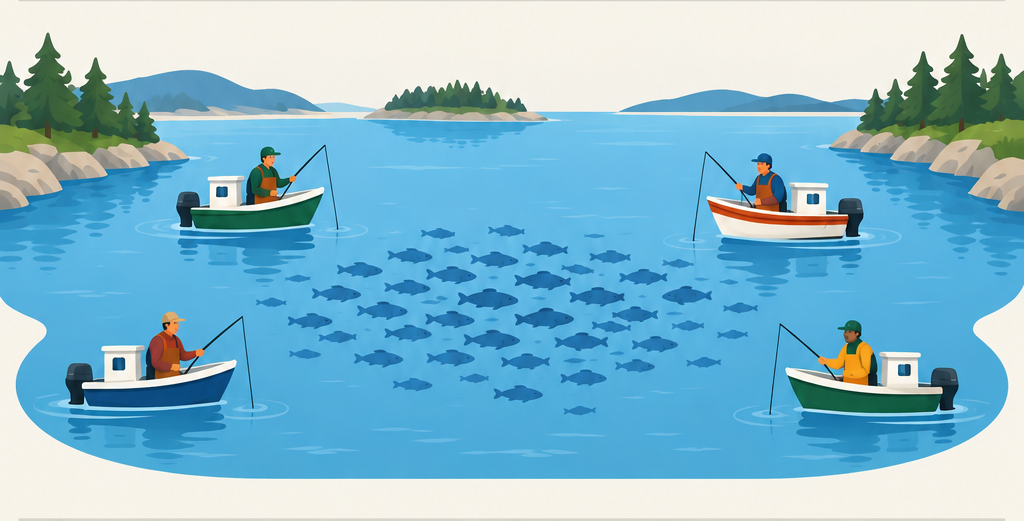
Four boats fishing from one shared bay.

All boats in your group fish from one bay.
Each boat privately chooses 0–5 fish.
No boat can stop another boat or set another boat’s catch.

\[ F_{t+1}=F_t+2n-H_t. \]

After Year 2, each fish left is worth 4 points, divided equally among the boats.

🤝 Fishing Setup 3: Group Limit, No Checks

Four boats fish in a shared bay with an unattended catch-limit sign at the dock.

The shared fish stock restarts.
Use your group’s maximum of 1, 2, or 3 fish per boat.
Keep the same group maximum for Setups 3–5.
Your catch is recorded, but there is no check or point deduction here.
You may choose 0–5 fish, including a catch above the agreement.
After Year 2, each fish left is worth 4 points, divided equally.

🎲 Fishing Setup 4: Group Limit, Random Checks

A dock inspector checks catches from boats returning from the shared bay while other boats continue fishing.

The shared fish stock restarts.
Use the same group maximum from Setup 3.
You may still choose any catch from 0–5 fish.
After all boats submit, the group-year has a 50% chance of being checked.
If checked, you lose 6 points per fish above the group maximum.
The check is revealed only after the group-year closes.
Every caught fish still affects the dock price and fish stock.

🛑 Fishing Setup 5: Limit Enforced at the Dock

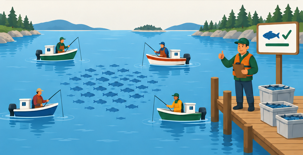
Four boats fish in a shared bay while a dock checker enforces the group maximum.

The shared fish stock restarts.
Use the same group maximum from Setup 3.
The dock rejects a catch above that maximum.
After Year 2, each fish left is worth 4 points, divided equally.

The limit changes which catches the dock accepts.

It does not change the stock equation.

🎟️ Your Total Game Score

Your total game points equal:

\[ \text{catch points from 10 choices} -\text{inspection penalties} +\text{5 ending-stock bonuses}. \]

In Your Own Pond, you receive the full value of the fish left in your pond.
In all four Shared Bay setups, the group divides the ending-fish value equally.

Each fish left after Year 2 is worth 4 points before the setup’s allocation rule is applied.

🏆 Prize Drawing

Students with ten accepted choices and a complete, consistent group record are eligible for the drawing.
The instructor randomly draws two eligible boat codes.
Every eligible boat code has the same chance of being drawn.
Your total game points determine the payment if your code is selected.

\[ \text{payment}=\max\left(\$0,\min\left(\$10,\frac{\text{total points}}{30}\text{ dollars}\right)\right). \]

For example, 210 points pays $7.00, and 300 points or more pays $10.

📱 Submit and Wait for the Instructor

Wait until the instructor announces the setup and year.
Use the matching Classwork 3 submission block.
Confirm your boat code, group, group size, and group maximum when shown.
Choose privately and submit only your catch.
Wait while the other boats submit.
The instructor reveals group catch, dock price, fish left, and any Setup 4 check.
The stock keeper records the announced results.

Corrections and backup

Before your group moves to the next year, you may resubmit; the latest accepted choice counts.
After a Setup 4 check is revealed, that group-year is closed.
If your device cannot submit, tell the instructor and use the paper backup.

🔍 What Changed Across the Five Setups?

How did having your own pond change what you wanted to catch?
Did a group agreement change catches when no check affected points?
Did a possible check change choices before its result was known?
How did immediate dock enforcement change choices?
Which differences may reflect the setup itself?
Which differences may reflect learning from earlier rounds?

🏞️ Property Rights, Open Access, and Resource Institutions

Rights and access rules shape incentives and resource use

🌐 External Costs and Resource Governance

An external cost arises when a resource user’s decision affects others, but the user does not bear the full consequence.
In the Shared Bay, one boat’s extra catch reduces the fish and future bonus available to every other boat.
Property rights define which decisions each user may make and which consequences that user must bear.

A resource institution must answer:
- Who may use the resource?
- Who may exclude others?
- Who receives the benefits and bears the costs?
- Who may transfer a right?
- Who can monitor and enforce the rule?

🔑 Effective Property Rights

Characteristic	Meaning
Exclusivity	The owner or user receives the benefits and bears the costs
Transferability	Rights can move voluntarily from one owner to another
Enforceability	Rights are protected against seizure or encroachment

In economics, property rights are a bundle of entitlements governing resource use.

Rights may belong to individuals, a defined group, or the state. Efficiency weakens when important costs remain outside the right holder’s decision.

🧩 Rivalry and Excludability

	Excludable	Difficult to exclude
Rival	Private good (timber)	Common-pool resource (fishery, aquifer)
Non-rival	Club good (gated park)	Public good (biodiversity, climate stability)

Rivalry: one person’s use reduces the amount or quality available to others.

Excludability: access can be limited to authorized users at reasonable cost.

🏛️ Four Governance Regimes

Regime	Who controls access?
Private property	An individual or firm
State property	A public authority
Common property	A defined user community
Open access	No actor exercises effective exclusion

Common property has rules and a defined group of users. Open access lacks effective exclusion.

How the experiment fits

Our classroom Shared Bay has a fixed group, so it is not literal open access.
It isolates the incentive created when several boats take fish from one stock.
The open-access model later adds entry by additional boats.

🤝 Common Property: Success and Failure

Case: Swiss Alpine Meadows (Common Property Success)

Grazing treated as common property for centuries.
User associations set stocking rules; stable membership fostered reciprocity and trust.
Outcome: Overgrazing discouraged; compliance high; sustained yields.

Case: Mawelle, Sri Lanka (Governance Breakdown)

Initially: Rotating rights over fishing spots/times ensured equity and protected stocks.
Later: Population growth + outsiders eroded cohesion; rules became unenforceable.
Outcome: Overexploitation and lower incomes.

Success ingredients: reciprocity, stable membership, transparent rules, graduated sanctions, local monitoring, compliance.

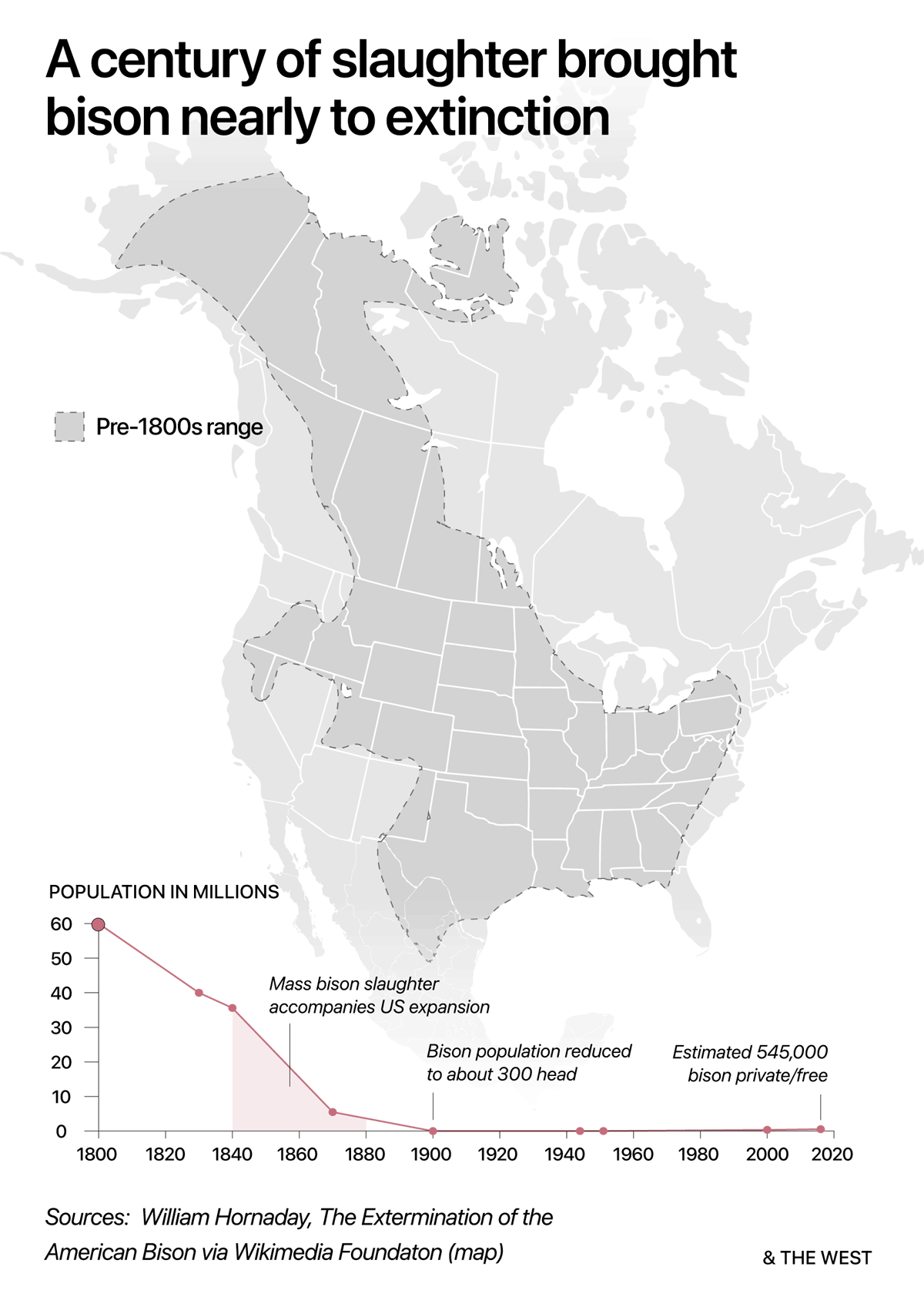
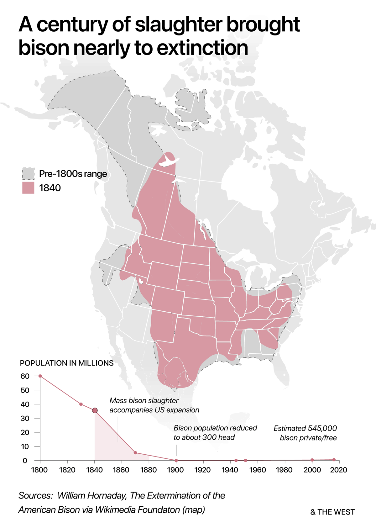
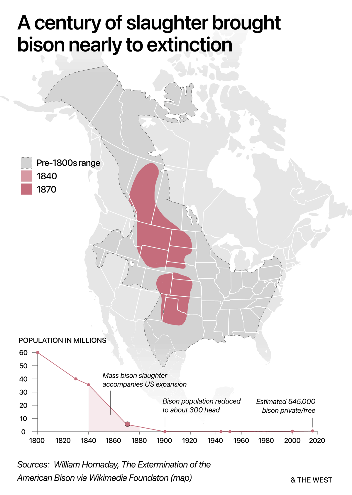
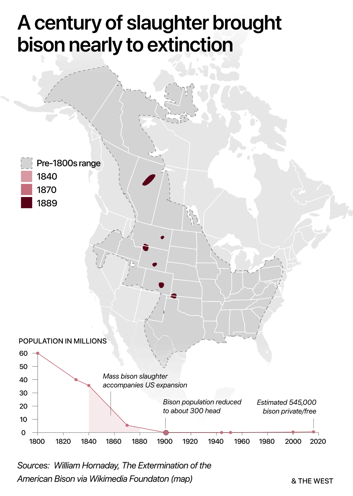
🦬 American Bison as a Common-Pool Example

Early U.S. period:
- Abundant bison; unrestricted hunting did not impose noticeable scarcity costs.
As demand/technology rose:
- Scarcity emerged; each hunter’s effort reduced others’ catch per unit effort.

Open access + scarcity ⇒ escalating harvest effort, falling stocks, near-extinction.

📈 Total Framework

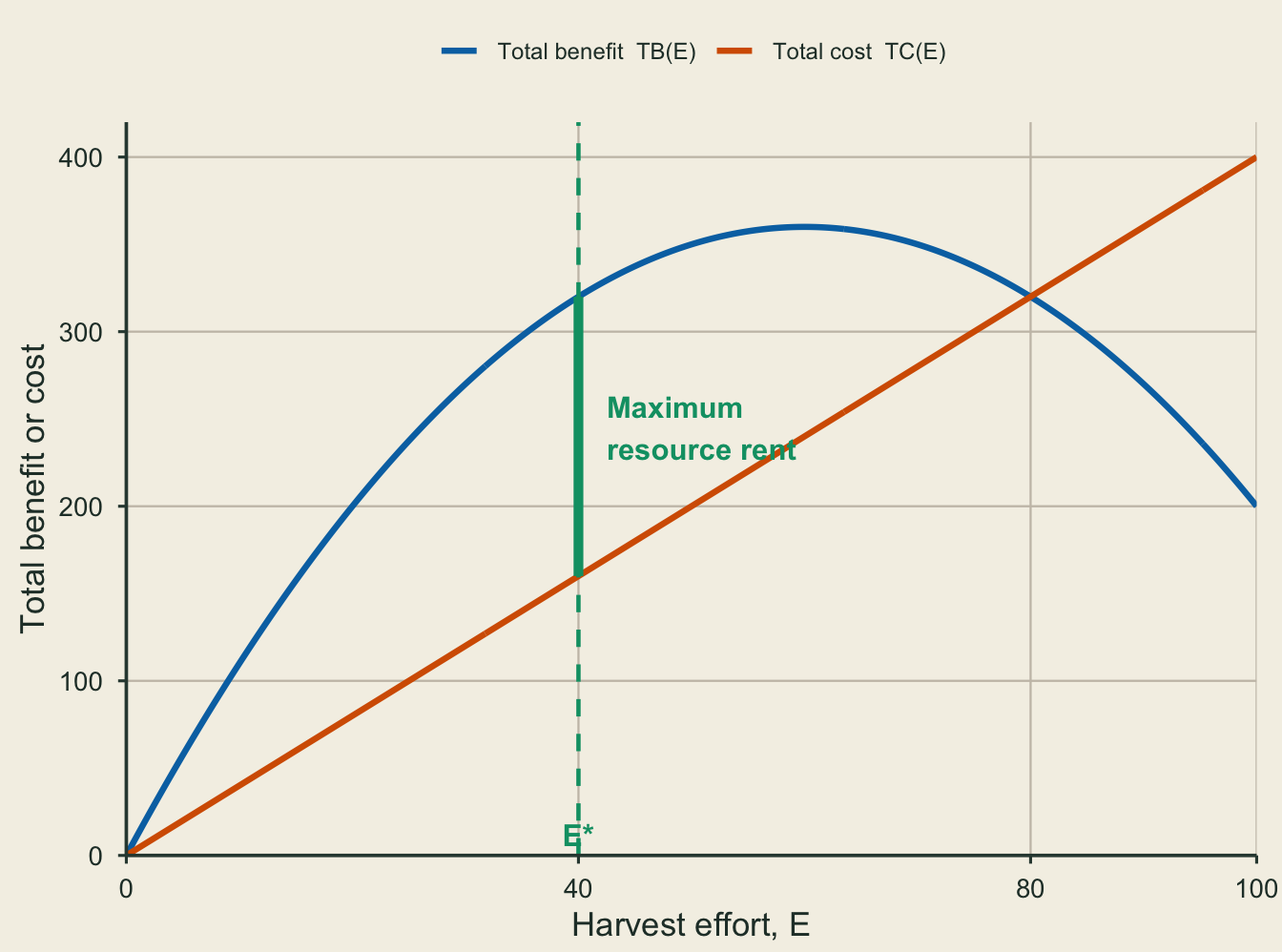
Total benefit and total cost as functions of harvest effort. The efficient effort maximizes the vertical resource-rent gap.

Total Surplus (Profit) $TS(E) = TB(E) - TC(E)$.
Total Benefit (Total Revenue) $TB(E)$: increase with effort at a diminishing rate.
Total Cost $TC(E)$: increases with effort $E$ (linear if marginal cost $c$ is constant).
Efficient effort $E^{*}$: maximizes the vertical gap between $TB$ and $TC$.

📉 Marginal Framework

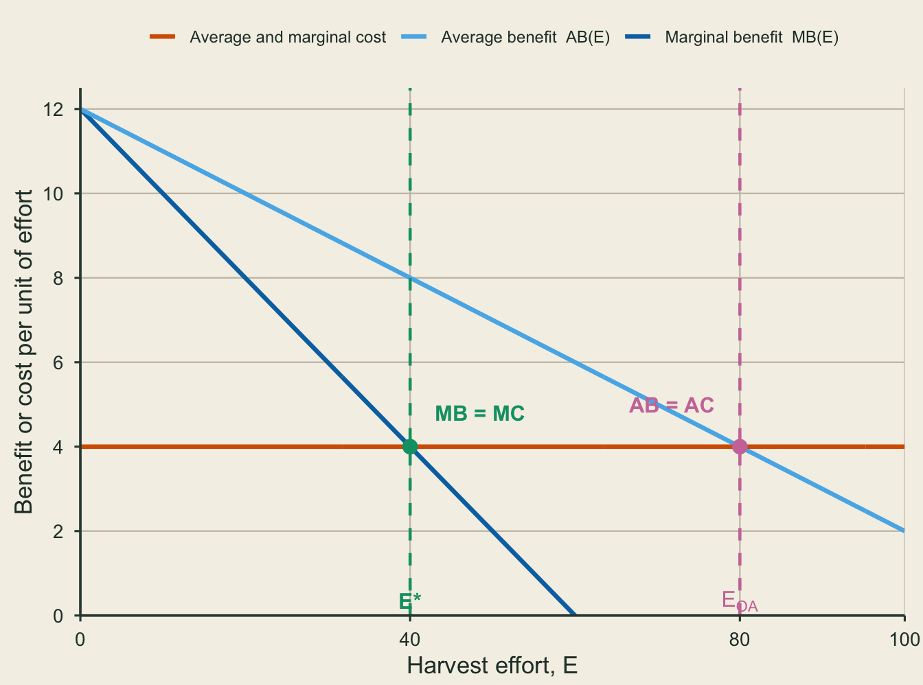
Marginal and average benefits with constant marginal and average cost. Efficient and open-access effort are marked.

Marginal Benefit $MB(E) = \frac{dTB}{dE}$ declines as stock falls with effort.
Marginal Cost $MC(E)$ (e.g., constant $c$).
Efficiency: $MB(E^{*}) = MC(E^{*})$.
Two panels are equivalent representations of the same optimum.

🎯 Efficient Effort $E^{*}$

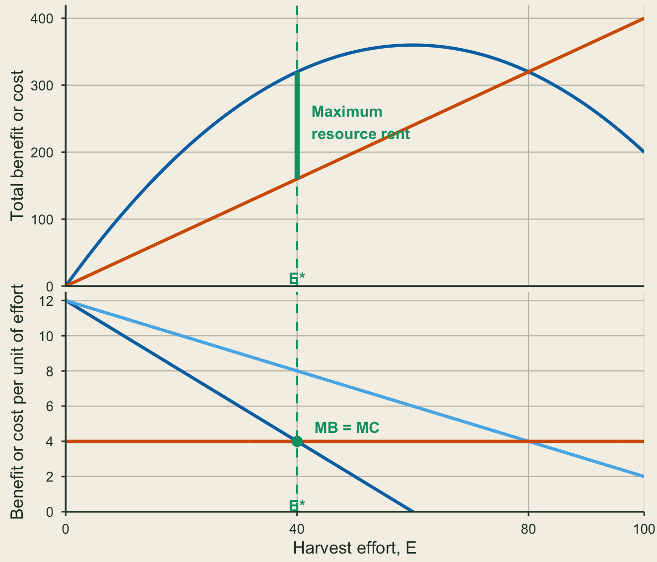
Two vertically stacked ggplot panels share an aligned harvest-effort axis. The top panel shows the efficient effort at the maximum gap between total benefit and total cost. The bottom panel shows marginal benefit equal to marginal cost at the same effort.

Top panel: $E^{*}$ maximizes the resource rent, $TB-TC$.
Bottom panel: the same effort satisfies $MB=MC$.
At $E^{*}$, the last unit of effort adds as much benefit as it costs.

🚪 Open-Access Effort $E_{OA}$

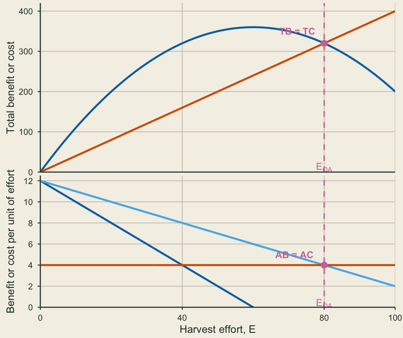
Two vertically stacked ggplot panels share an aligned harvest-effort axis. The top panel shows total benefit equal to total cost at open-access effort. The bottom panel shows average benefit equal to average cost at the same effort.

Top panel: $TB=TC$, so total surplus is zero.
Bottom panel: free entry stops where $AB=AC$ because each user earns zero profit.

Because $AB=TB/E$ and $AC=TC/E$, the conditions are equivalent:

\[ \begin{aligned} AB=AC &\;\Longleftrightarrow\; TB=TC \\ &\;\Longleftrightarrow\; TS=0. \end{aligned} \]

⚠️ Open-Access Overuse: Tragedy of the Commons

Unlike the classroom Shared Bay, open access also allows free entry.
No exclusion ⇒ no one can secure surplus.
Each user ignores the stock-scarcity cost: the stock externality that current effort imposes on other users now and on future resource users.
With free entry, effort keeps expanding until per-user profit $=0$.
- This drives total economic rent to zero.
Why does effort go too far?
- When total benefits ($TB$) flatten under diminishing returns, the average benefit ($AB$) stays above the marginal benefit ($MB$).
- Users enter while $AB>AC$, even after $MB<MC$, so effort rises past the efficient level.
Result: $\;\;E_{OA} > E^{*}$ and all rents are dissipated.

🎁 Public Goods and Underprovision

In competitive markets, demand = willingness to pay (WTP) for private goods.
For public goods, individual WTP understates marginal benefit (MB) because people can consume even if they pay less (or nothing).
Result: Free riding → $\text{(Total Voluntary Funding)} \,<\,\text{(Cost)}$ → Underprovision.

Note

Market failure here is on the demand side, unlike common-pool overuse, which arises from decisions on the production side.

➕ Vertical Summation of Public-Good Benefits

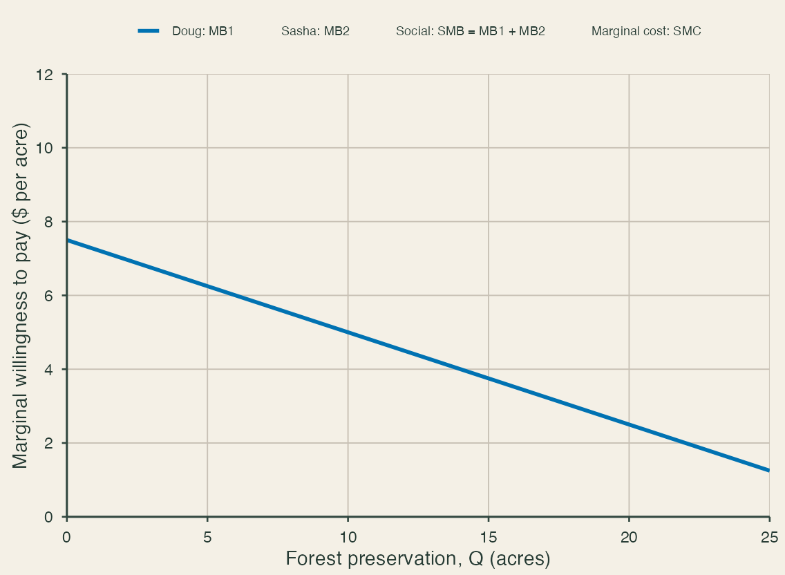
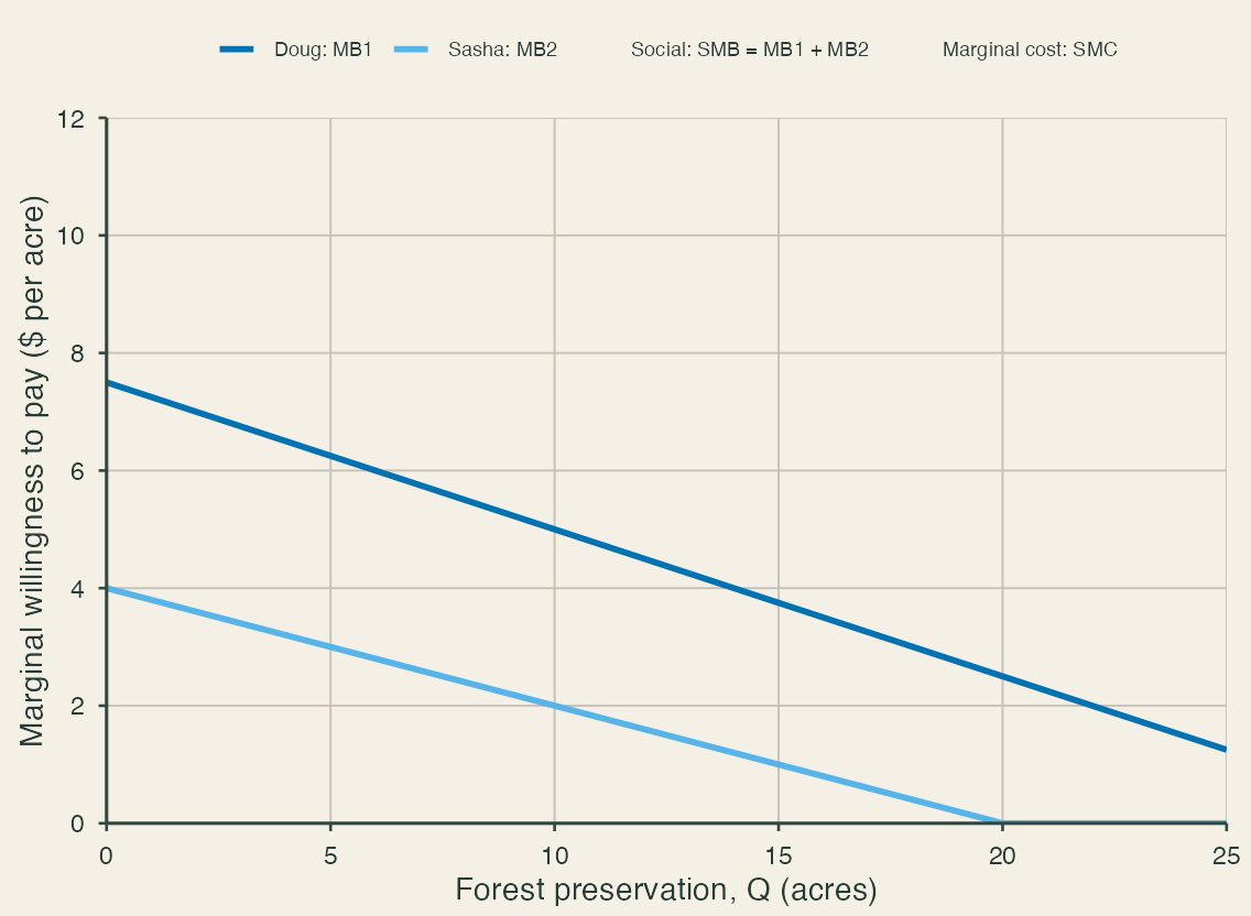
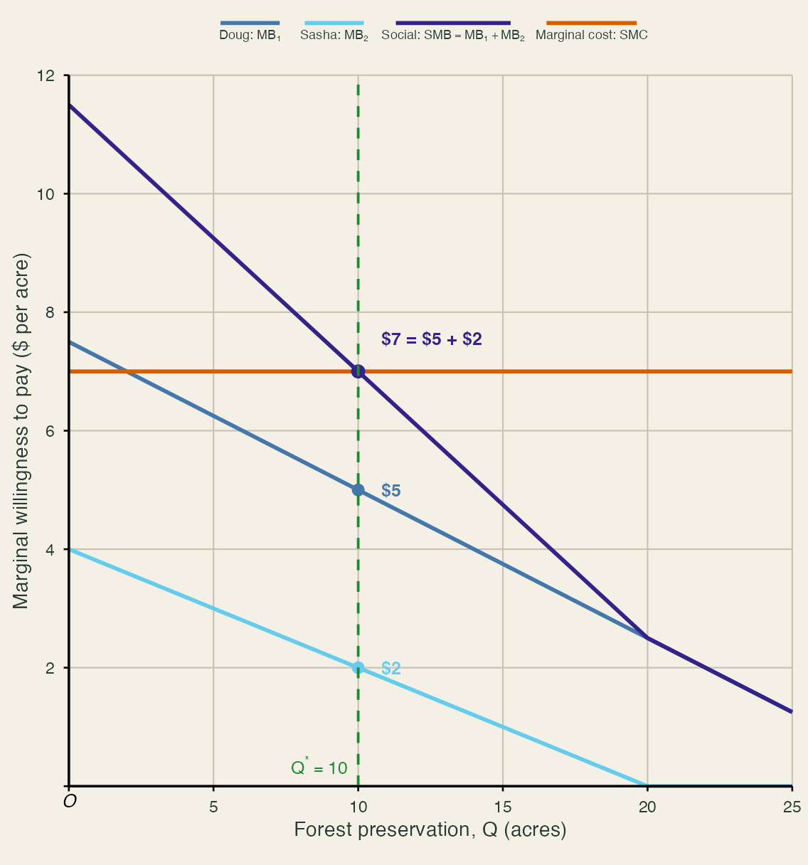
1. Doug’s marginal benefit

2. Add Sasha’s marginal benefit

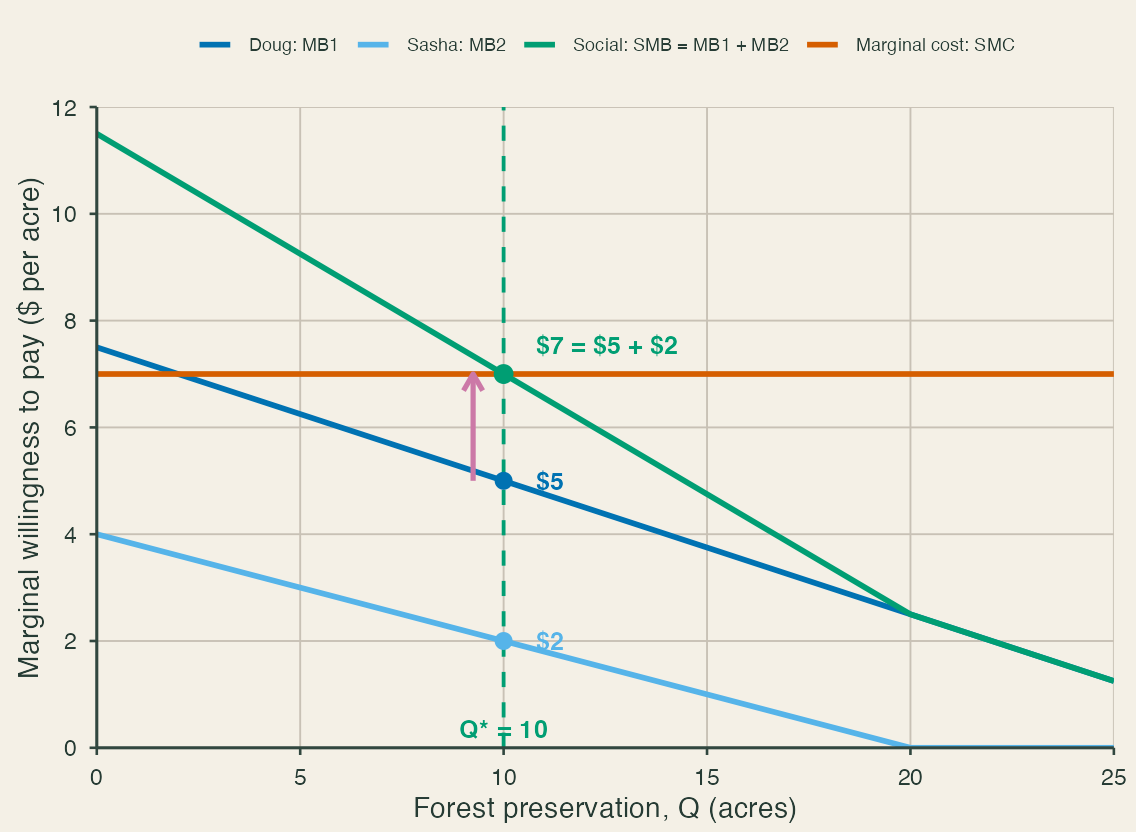
At $Q=10,$their values are $5 and $2.

3. Sum the benefits vertically

\[ SMB(Q)=MB_D(Q)+MB_S(Q) \]

At $Q=10,$

\[ SMB=\$5+\$2=\$7. \]

4. Compare $SMB$with $SMC$

At $Q=10.$

\[ SMB=SMC=\$7. \]

Therefore, $Q^{*}=10.$

💵 Funding the Efficient Quantity

At $Q^{*}=10$, total cost is $70. Efficiency determines how much to provide. Financing determines who pays.

Financing rule	Example	Main consideration
Uniform tax	Doug pays $35 and Sasha pays $35	Simple, but ignores benefit differences
Benefit-based shares	Doug pays more because his marginal benefit is higher	Better aligned with benefits, but true willingness to pay is hard to observe
Ability-to-pay	Contributions rise with income	Addresses equity, but does not track individual benefits

🧭 Institutional Paths Toward Efficiency

Ill-defined rights can separate private choices from collective costs and benefits. Two institutional pathways can address this gap:

Pathway	Main mechanism	Best suited to
Judicial liability	Compensation for demonstrated harm after the fact	Distinct events with identifiable sources and victims
Legislative and executive regulation	Rules, limits, standards, and information requirements before harm occurs	Repeated or diffuse harms involving many parties

Both pathways can fail when information or enforcement is weak.

⚖️ Judicial Liability: Mechanism

How it works

After harm occurs, liability law requires the responsible party to pay compensation that corresponds to the damage.
Strict liability can apply even without negligence or fault, especially for abnormally dangerous activities.
Negligence asks whether the party exercised the legally required level of care.

Oil-spill example

A company expects to pay for cleanup and compensate injured parties if a spill occurs.
When prevention costs less than expected cleanup and damages, prevention becomes privately valuable.
Liability internalizes the external cost, moving the company’s choice closer to the efficient outcome.

⚠️ Limits of Judicial Liability

Courts must identify the responsible party and estimate the damages.
Transaction costs are the costs of reaching and enforcing a fair outcome. Examples include court time, legal fees, and expert testimony.
These costs rise with many parties or recurring disputes.
One general rule can reduce these costs in recurring cases.

Contrast: Courts can more easily assign liability for a single oil spill with a clear source than for ongoing pollution from many sources.

Coase Theorem

When property rights are clearly defined and transaction costs are low, affected parties can bargain toward an efficient outcome.
- The initial assignment of rights still determines who pays and who receives compensation.
Example: A paper mill and downstream fishers can bargain over pollution reduction or compensation when their rights concerning water quality are well-defined and reaching agreement is inexpensive.

🚧 Regulation: Activity and Access

Rule	What it controls	Natural-resource example
Activity limit	The quantity of emissions, withdrawals, or harvest	Catch quota or groundwater-pumping limit
Spatial or timing rule	Where and when use may occur	Seasonal closure, no-take zone, or wetland setback
Access or entry rule	Who may use the resource	Limited permits or grazing leases

Setup 3: the group states a limit, but no check affects points.
Setup 4: monitoring is incomplete, and a possible penalty follows a detected excess catch.
Setup 5: the dock enforces the catch limit immediately.

Effective rules need measurable limits, credible monitoring, and enforceable penalties.

🧾 Regulation: Practice and Information

Rule	Purpose	Natural-resource example
Input or process standard	Requires protective practices or prohibits damaging methods	Fishing-gear restriction or forestry best-management practice
Safety or licensing rule	Sets operator qualifications and operating conditions	Resource-use permit or spill-response plan
Disclosure, certification, or labeling	Makes environmental performance visible	Pollution-release reporting or sustainable-resource certification

Rent seeking

Rent seeking occurs when people or firms spend resources trying to shape a rule for their own gain instead of creating new value.
Example: A firm may lobby for a licensing rule that limits competitors or gives it favored access.
Weak information and enforcement can make this form of government failure more likely.