Lecture 5

Resource Allocation Over Time

Byeong-Hak Choe

bchoe@geneseo.edu

SUNY Geneseo

September 21, 2026

💵 The Discount Rate

❓ Resource Allocation across Generations

How should a limited natural resource be divided across generations?
How can we compare benefits and costs that occur at different dates?
What happens to prices and consumption as a resource becomes scarce?

🗓️ Values at Different Dates

Costs and benefits often occur at different dates.

Expressing amounts in real dollars removes inflation. It does not make a future dollar equivalent to a current dollar.

A positive discount rate reflects the return available elsewhere and the weight placed on earlier consumption.

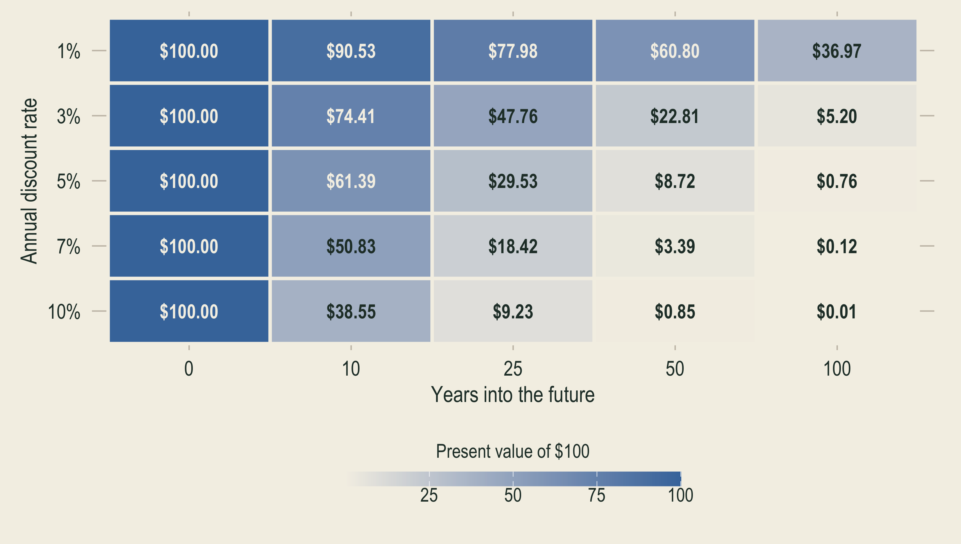
Discounting converts a future real amount into its present value.

🧮 Present Value

Let $X_t$ be an amount received in $t$ years and let $r$ be the annual discount rate.

\[ PV(X_t)=\frac{X_t}{(1+r)^t}. \]

Present value falls when the date moves farther into the future.

Present value also falls when the discount rate rises.

Use real future amounts with a real discount rate.

🔢 PV of $100 across Rates and Years

A heatmap shows the present value of 100 dollars at discount rates from 1 to 10 percent and horizons from zero to 100 years. Present value falls as the rate or time horizon increases. — Figure 1

🌎 A Long-Term Policy Example

Suppose a policy prevents $500 billion in climate damages 50 years from now.

Which present value uses a 2% rate, and which uses a 5% rate?

$185.8 billion
$43.6 billion

The future benefit is unchanged. The rate changes its present value and can change the policy decision.

🏙️ Quick Detour: Manhattan and Compounding

Suppose the often-cited $24 figure had instead been invested at an assumed annual return of 4.66% from 1626 to 2026.

Four hundred years of compounding gives

\[ FV_{2026}=\$24(1.0466)^{400}\approx\$1.96\text{ billion}. \]

Over 400 years, even a small change in the assumed return produces a very different future value.

This is a compounding illustration, not a historical appraisal of Manhattan land.

✌️ Quick Detour: The Rule of 72

The Rule of 72 estimates how long a value takes to double at a constant annual rate.

\[ \text{Years to double}\approx\frac{72}{r}, \]

where $r$ is written as a percentage rather than a decimal.

At 3% per year, doubling takes approximately 24 years.

The rule works best for moderate rates and provides intuition for compounding and discounting.

🧭 A Fixed Stock across Generations

🌍 Two Kinds of Resource Stock

This lecture focuses on nonrenewable resources, using neodymium as the main example.

Renewable resources regenerate through ecological processes.

Forests and fisheries can remain productive when harvest does not repeatedly exceed growth.
Renewable does not mean impossible to deplete.

Nonrenewable resources do not regenerate on a human time scale.

Oil, coal, and mineral deposits are examples.
One unit extracted today cannot also be used later.

🧲 Neodymium Model Setup

An educational illustration showing a mineral mine, neodymium-bearing ore, separated rare-earth oxide, and a permanent-magnet electric motor.

Resource: 250 model tons of recoverable neodymium in one known deposit
Use: permanent magnets in electric motors and some wind turbines
Market: magnet manufacturers’ WTP compared with marginal mining, separation, and processing cost
Time and stock: two periods, ten years apart, with one fixed stock and no discoveries
Benchmark: illustrative equations omit joint production, recycling, substitution, and environmental harm

📊 Neodymium Market Model

🧮 Current Demand and Supply

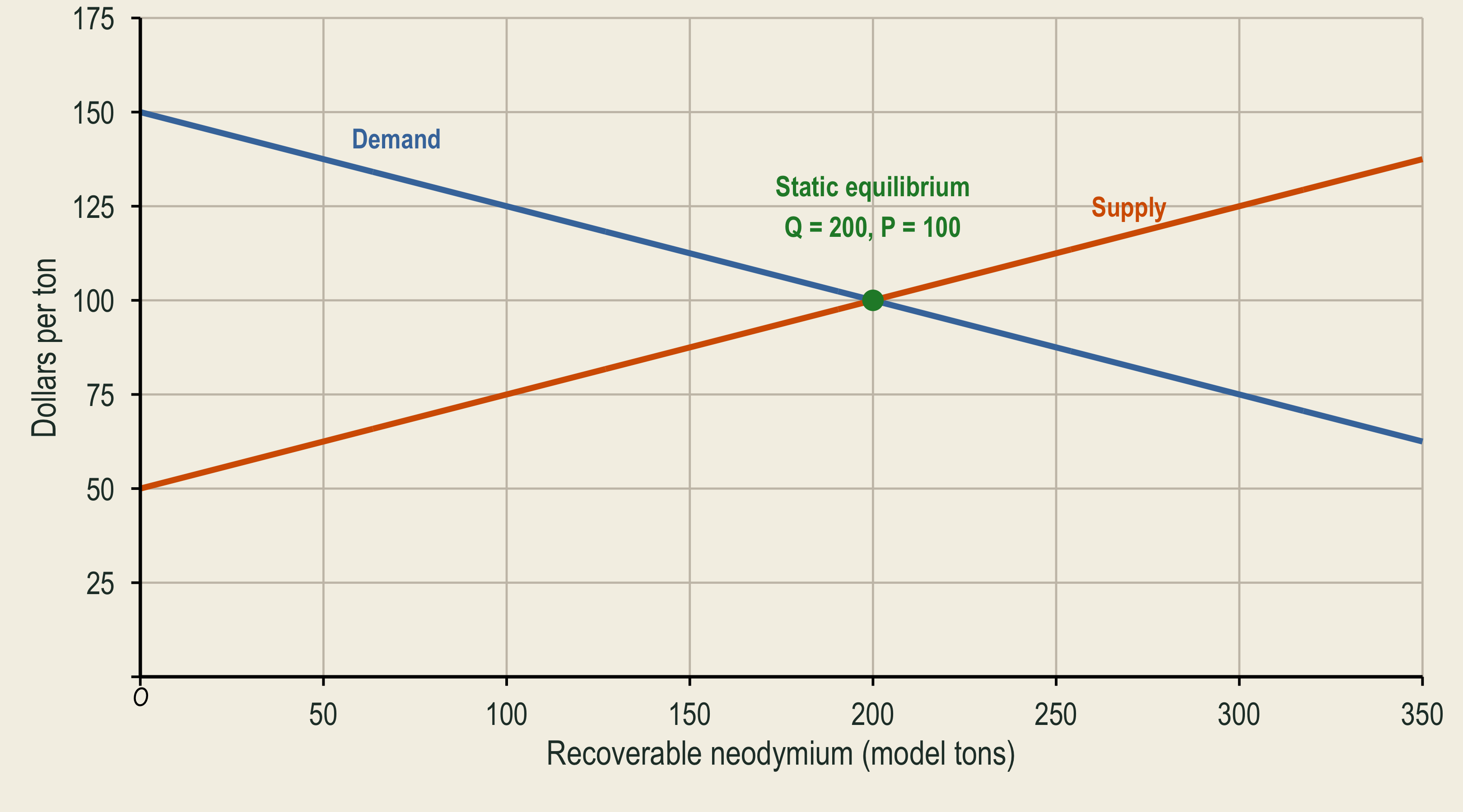
Demand:

\[ P_D=150-0.25Q. \]

Supply:

\[ P_S=50+0.25Q. \]

$Q$ is model tons of recoverable neodymium. $P$ is an illustrative price, not a market estimate.

Demand measures magnet manufacturers’ marginal willingness to pay. Supply measures marginal mining, separation, and processing cost.

⚖️ Static Neodymium-Market Equilibrium

Demand for recoverable neodymium slopes downward and supply slopes upward. They intersect at 200 model tons and 100 dollars per ton. — Figure 2

➖ Marginal Net Benefit

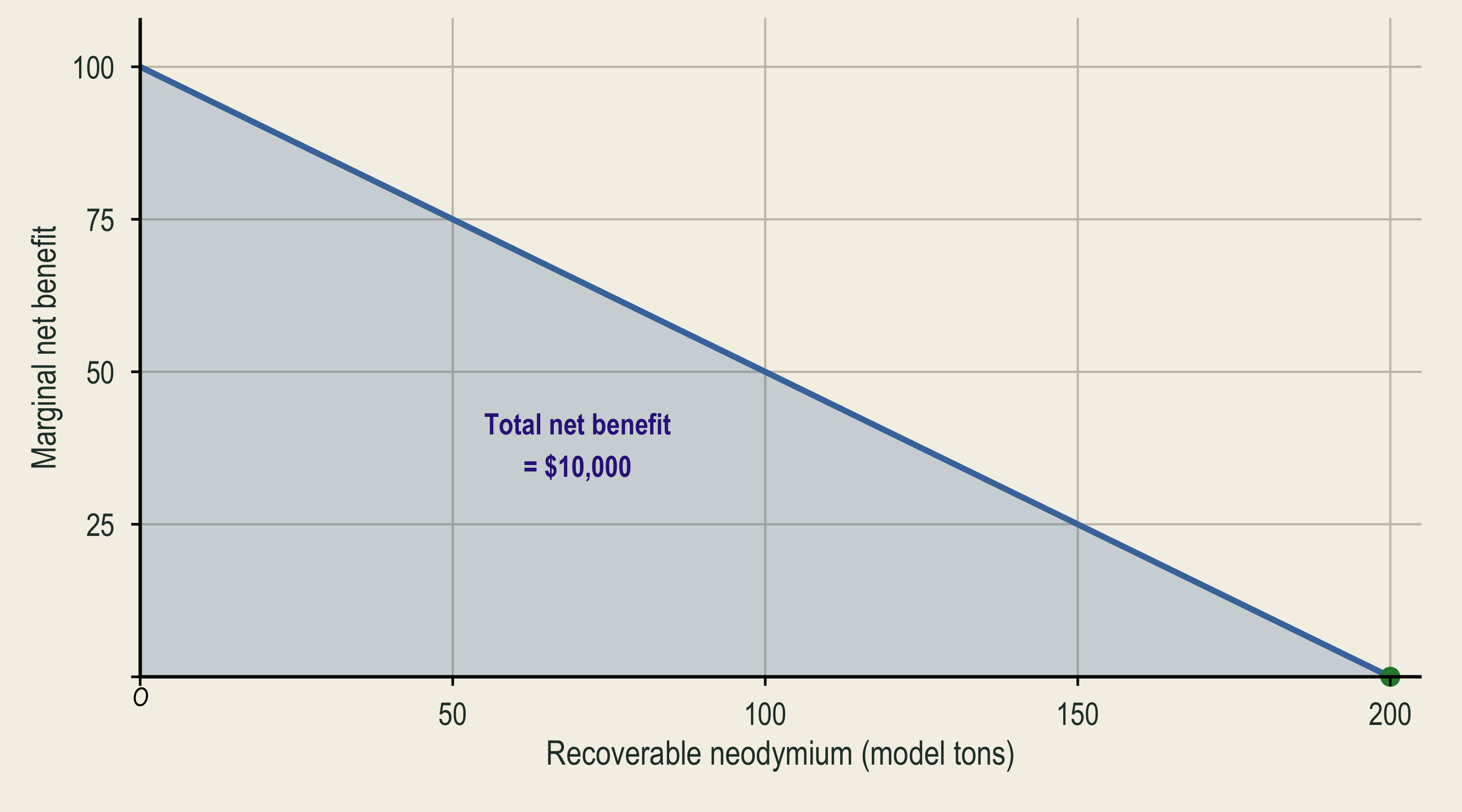
Marginal net benefit is marginal benefit minus marginal cost:

\[ MNB=P_D-P_S. \]

For this illustrative market,

\[ MNB=(150-0.25Q)-(50+0.25Q). \]

\[ MNB=100-0.5Q. \]

🔺 Total Net Benefit

Marginal net benefit falls from 100 to zero at 200 tons. The triangular area beneath the curve is 10,000 dollars. — Figure 3

🧾 Static Equilibrium

At $Q=200$,

\[ MNB=100-0.5(200)=0. \]

The area under MNB is total benefit minus total cost:

\[ TNB=\frac12(200)(100)=10{,}000. \]

A static equilibrium counts only present benefits and costs.

🕰️ Put Two Periods on One Clock

↔︎️ The Stock Constraint

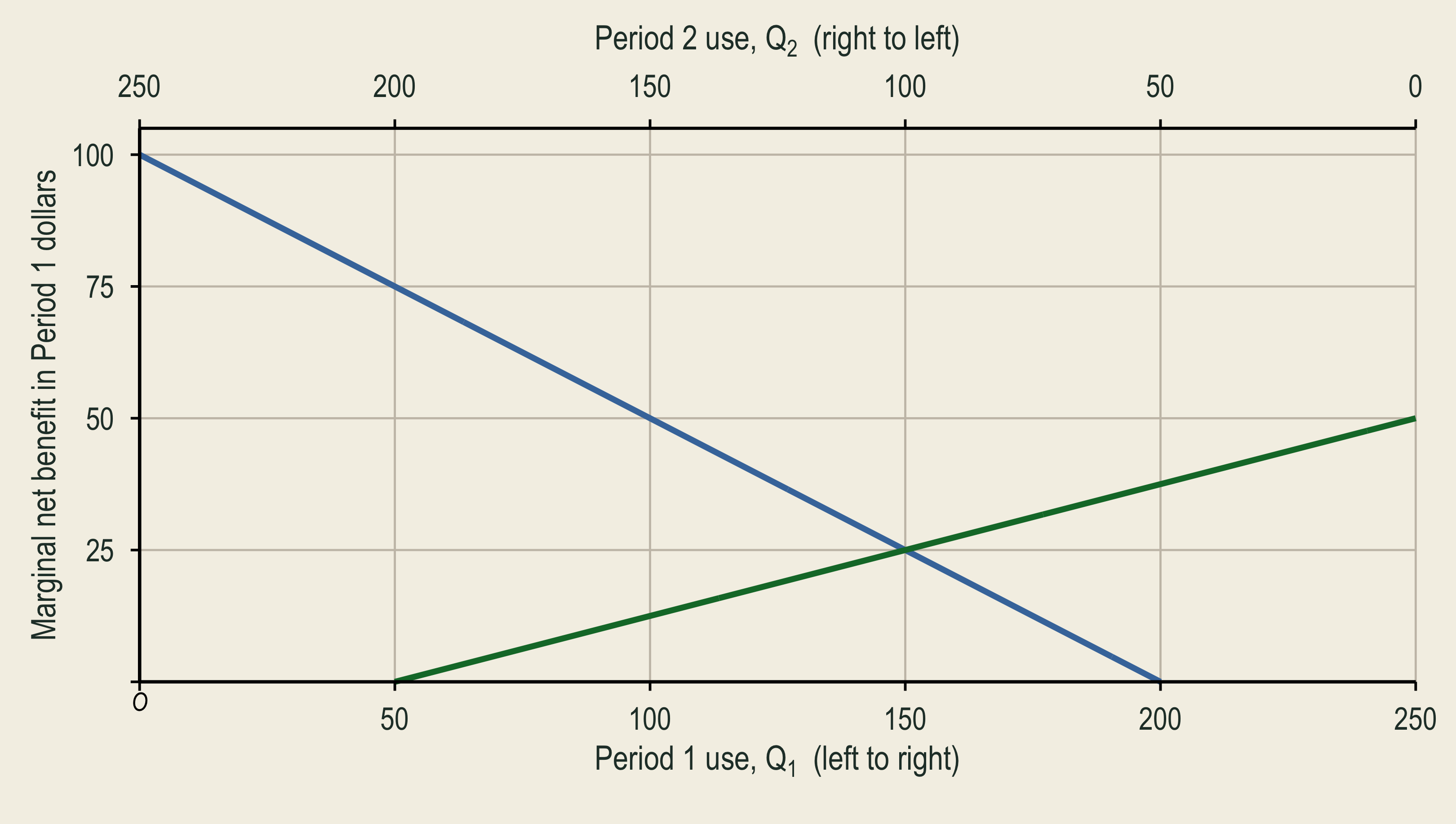
Suppose the known deposit contains 250 model tons of recoverable neodymium.

\[ Q_1+Q_2=250. \]

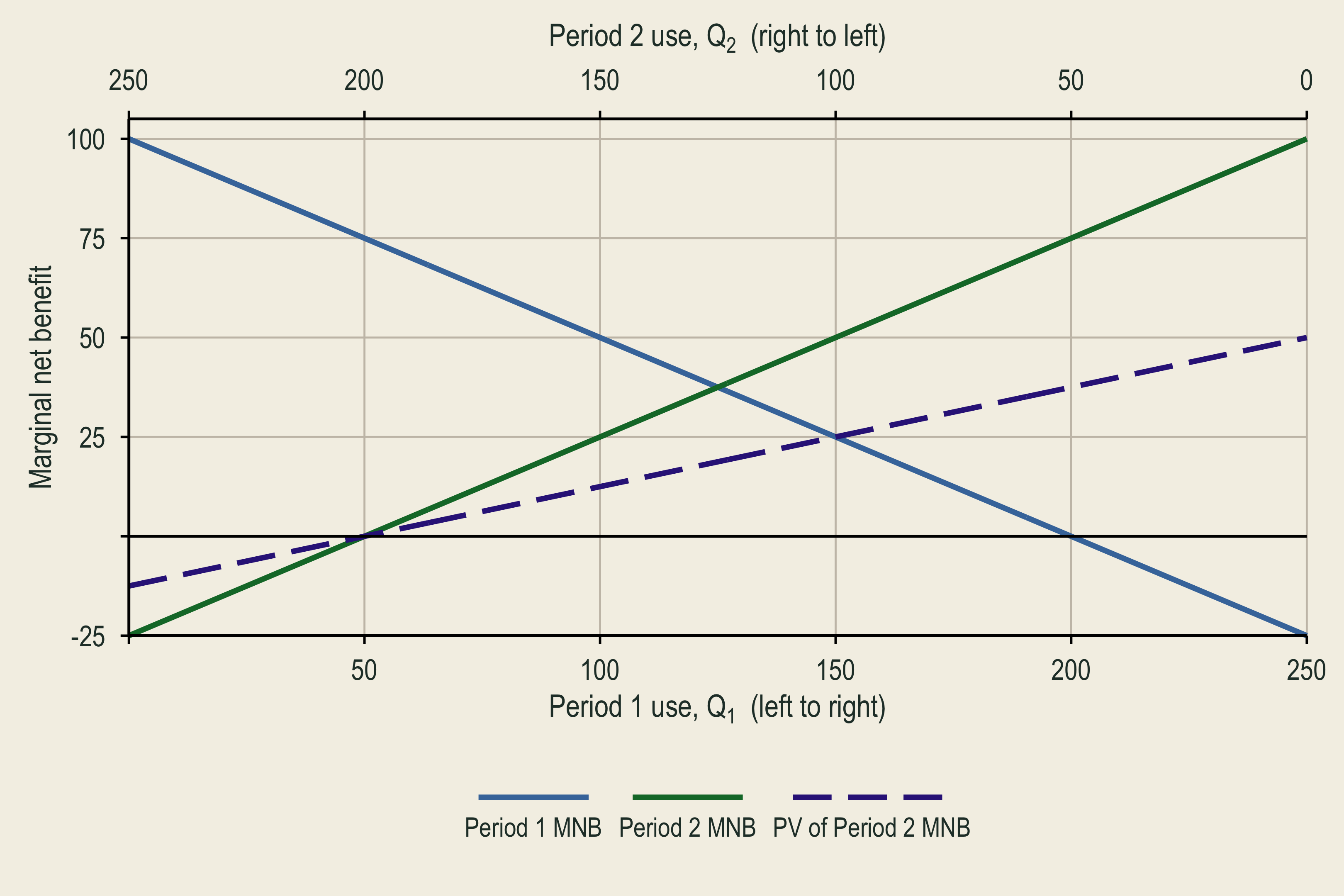
The two periods have the same undiscounted marginal net benefit:

\[ MNB_1=100-0.5Q_1, \]

\[ MNB_2=100-0.5Q_2. \]

🪞 The Mirror Axis

Period 1 marginal net benefit slopes downward. Period 2 marginal net benefit is mirrored, and its discounted value is lower. — Figure 4

⏳ Discount Period 2

The periods are ten years apart.

\[ (1.0725)^{10}\approx2. \]

Therefore,

\[ PV[MNB_2]\approx\frac{MNB_2}{2}. \]

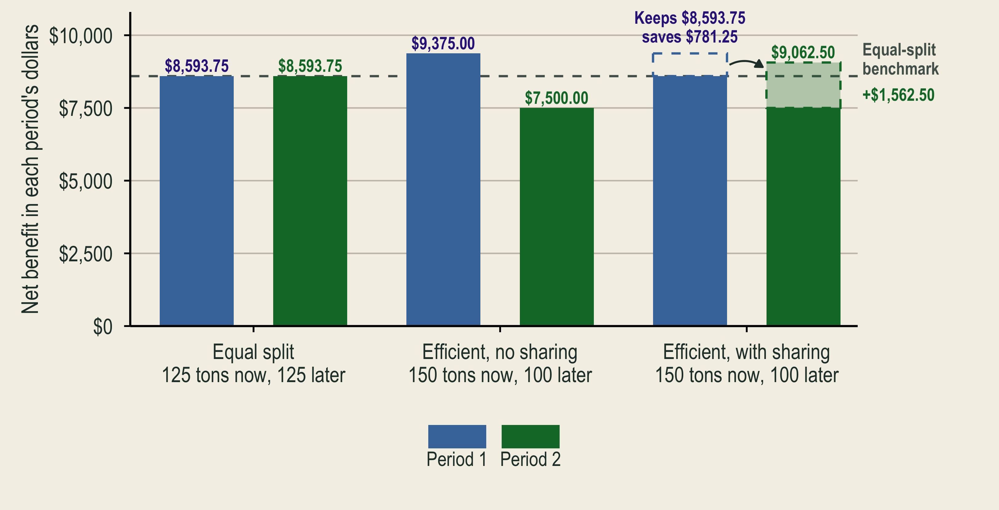
Discounting lowers every Period 2 marginal net benefit when measured in Period 1 dollars.

🎯 Dynamic Equilibrium

⚖️ Equal Values at the Margin

The efficient allocation satisfies both conditions:

\[ \begin{aligned} MNB_1 &= PV[MNB_2],\\ Q_1+Q_2 &= 250. \end{aligned} \]

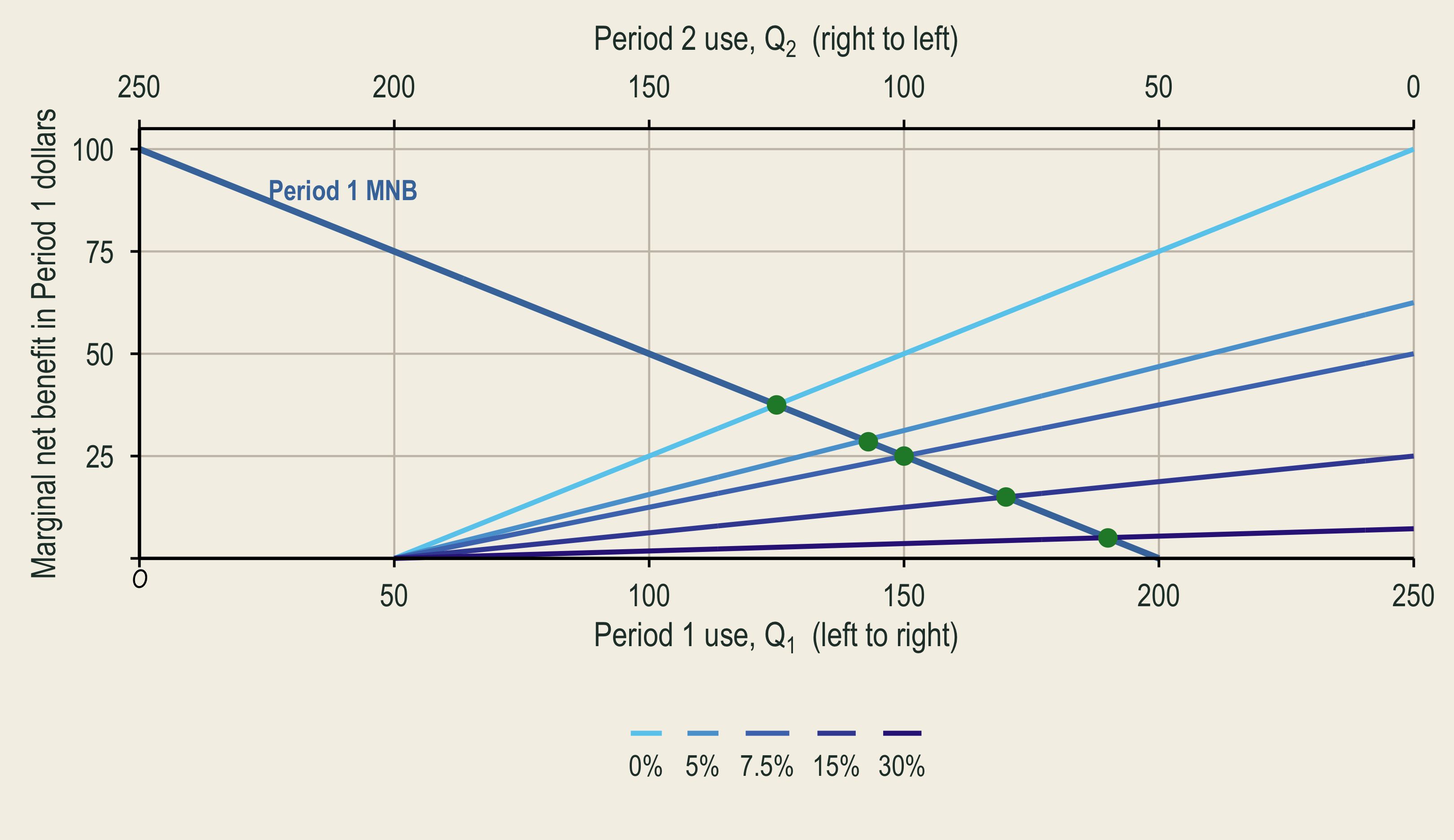
For example, consider $Q_1=125$ and $Q_2=125$:

Here, $MNB_1=37.50$ while $PV[MNB_2]=18.75$.

Moving a small amount of neodymium from Period 2 to Period 1 would therefore raise discounted total net benefit.

Using these two conditions, solve for $Q_1$ and $Q_2$.

🟢 The Optimal Allocation

Period 1 marginal net benefit and discounted Period 2 marginal net benefit cross at 150 tons now and 100 tons later. Areas A and B are shaded. — Figure 5

🔻 Too Much Current Use Loses Welfare

Period 1 marginal net benefit and discounted Period 2 marginal net benefit cross at the efficient allocation. — Figure 6

A dashed line marks an allocation of 200 tons in Period 1 and 50 tons in Period 2. — Figure 7

The allocation of 200 tons now and 50 tons later creates a red welfare-loss triangle labeled Net loss B 2. — Figure 8

🧭 Dynamic Equilibrium

A dynamic equilibrium counts current and future benefits and costs.

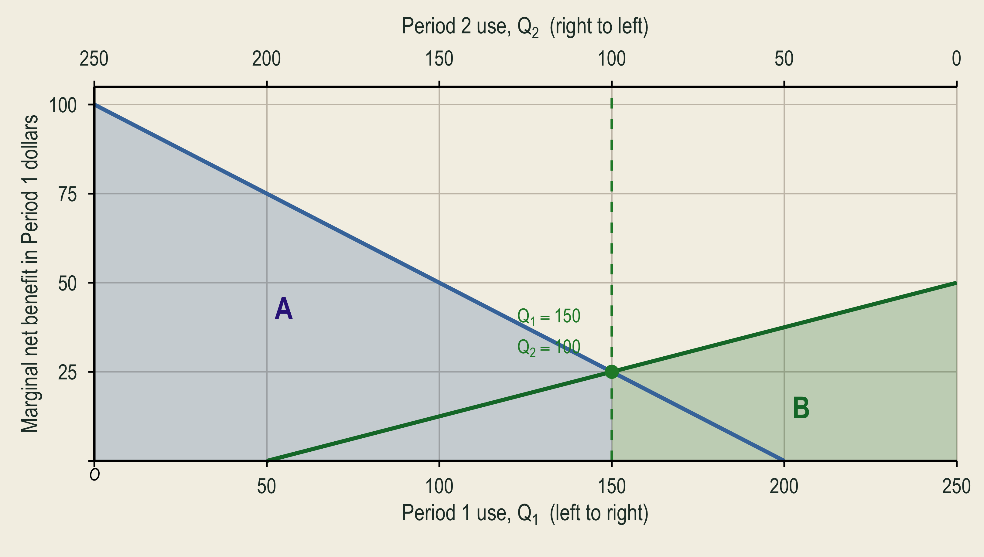
At the crossing,

present-value marginal net benefit is equal across dates;
the full stock is allocated; and
no reallocation can increase discounted total net benefit.

💎 User Cost and Depletion Policy

🕳️ Current Use Has a Future Opportunity Cost

User cost is the future opportunity lost when one more unit is extracted now.

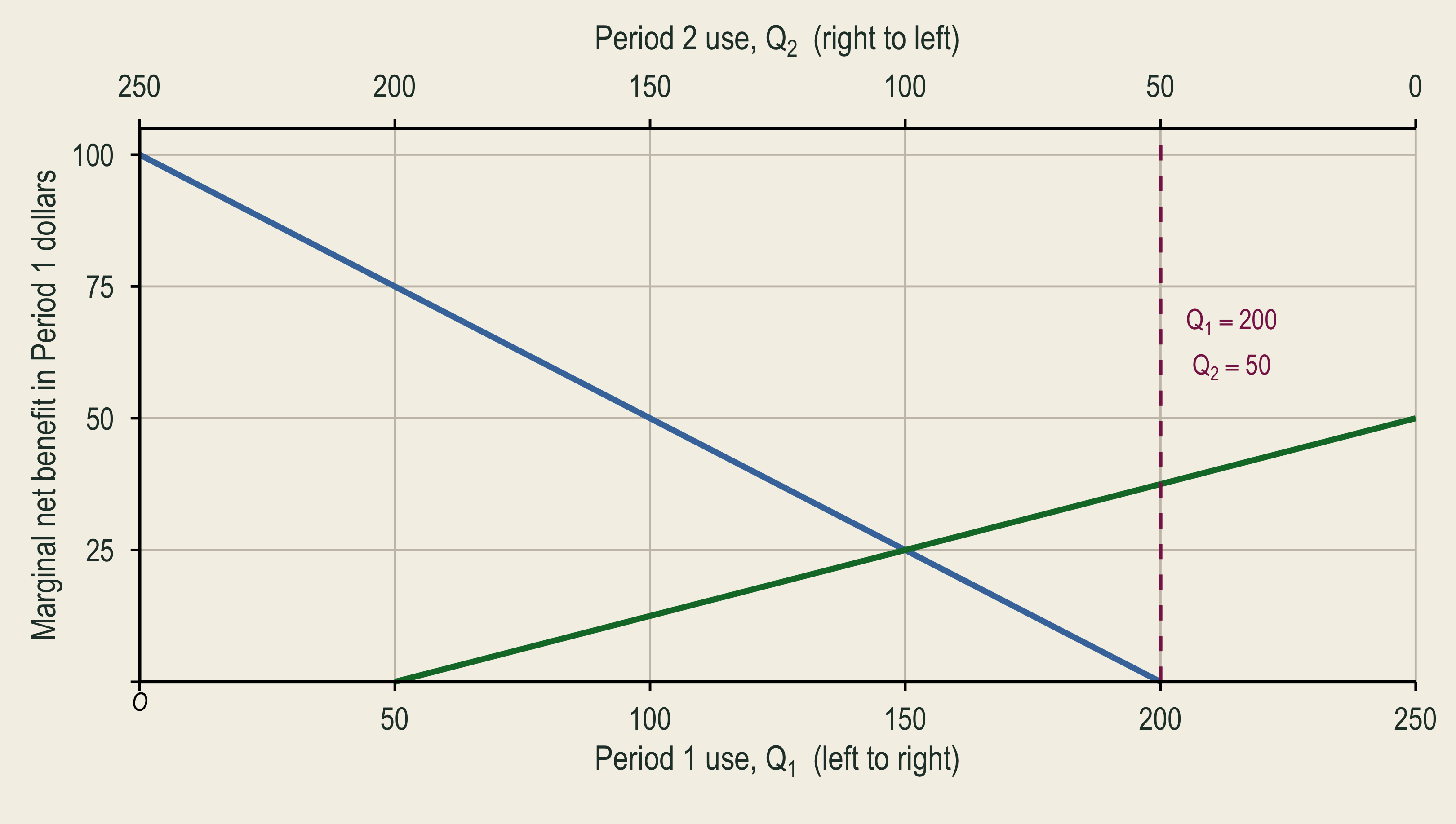
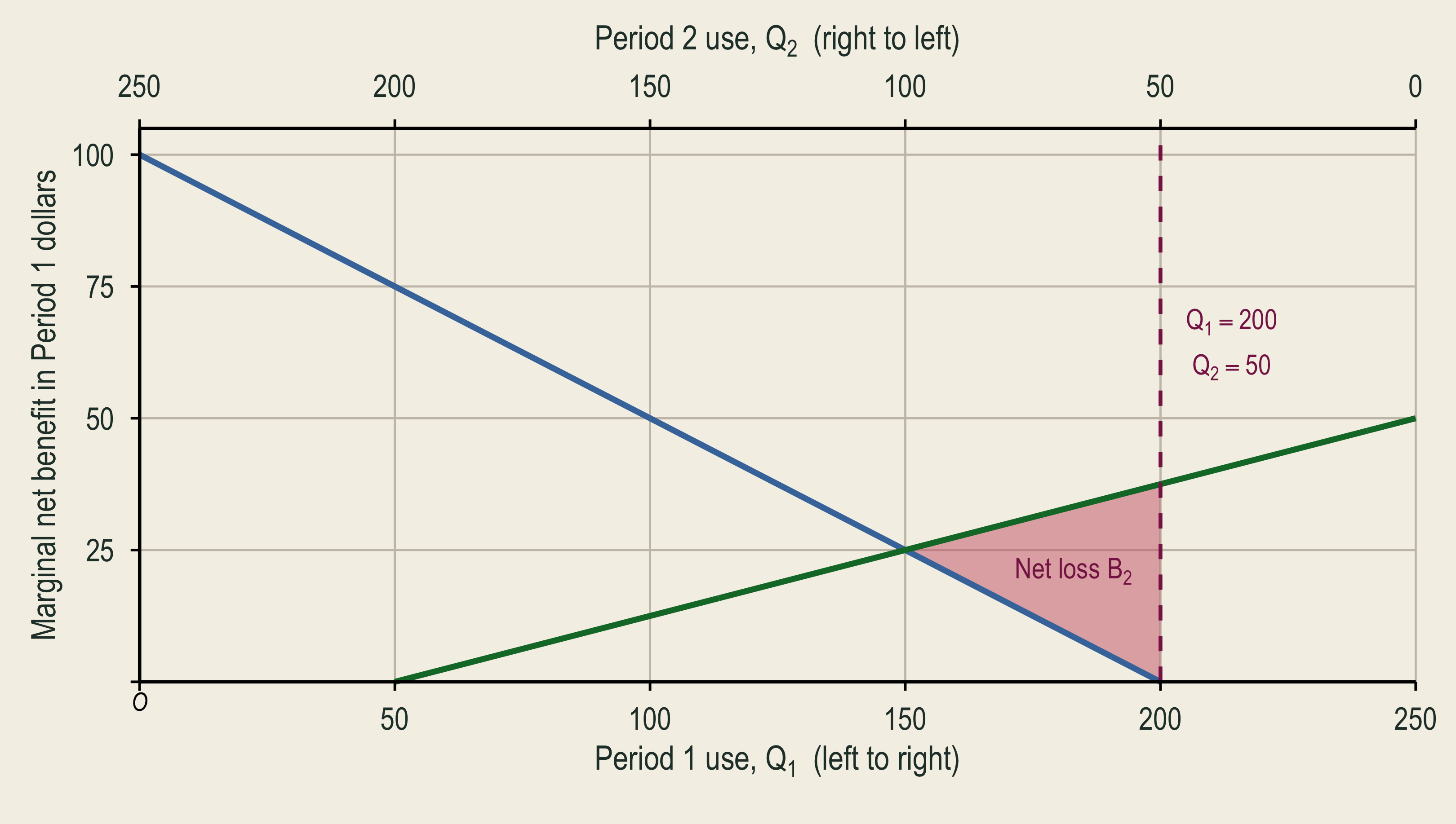
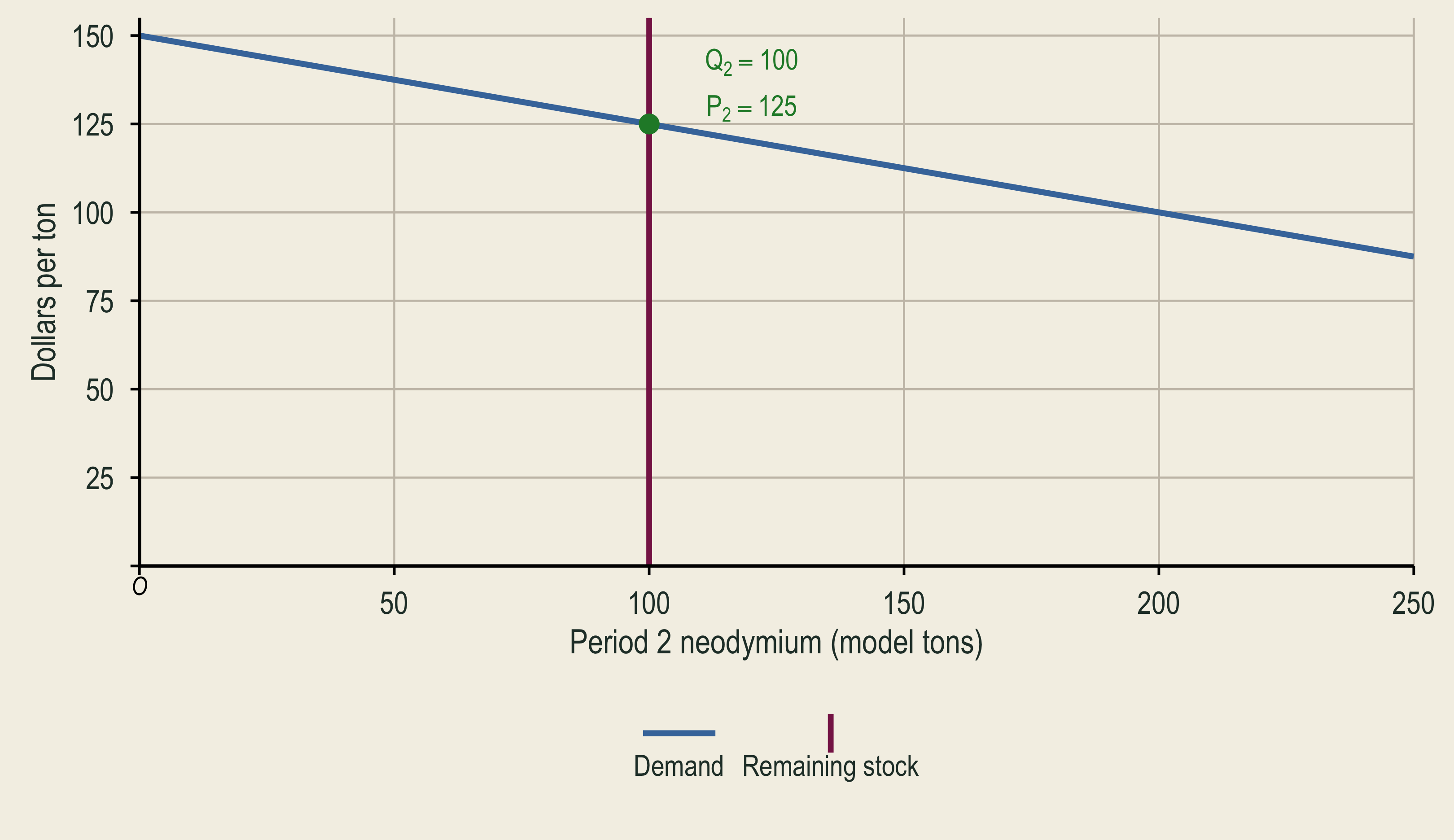
Period 2 would choose 200 tons in its static market.

If Period 1 uses more than 50 tons, fewer than 200 remain for Period 2.

From that point, another current ton displaces a desired future ton.

🧮 User Cost at the Efficient Quantity

From Period 1,

\[ MNB_1(150)=100-0.5(150)=25. \]

From Period 2,

\[ PV[MNB_2(100)]=\frac{100-0.5(100)}{2}=25. \]

The equilibrium user cost is $25 per ton.

🇯🇴 Mineral Depletion and Future Income in Jordan

NASA satellite image of a phosphate mine in Jordan

Jordan mines phosphate and potash, two nonrenewable minerals used in fertilizer.
Extraction earns current income but gives up future income. User cost measures this tradeoff.
Using a 3% discount rate, one study estimated about $550 million in user costs during 2002–2010.
That estimate was about 20% of mining profits over the same period.
Reinvesting this portion of mineral income can build education, infrastructure, or renewable natural capital for future generations.

🧾 Internalize User Cost

Demand, extraction cost, social cost with user cost, and supply with a 25 dollar tax meet at the efficient Period 1 outcome of 150 tons and 112.50 dollars. — Figure 9

💵 The Resource Depletion Tax

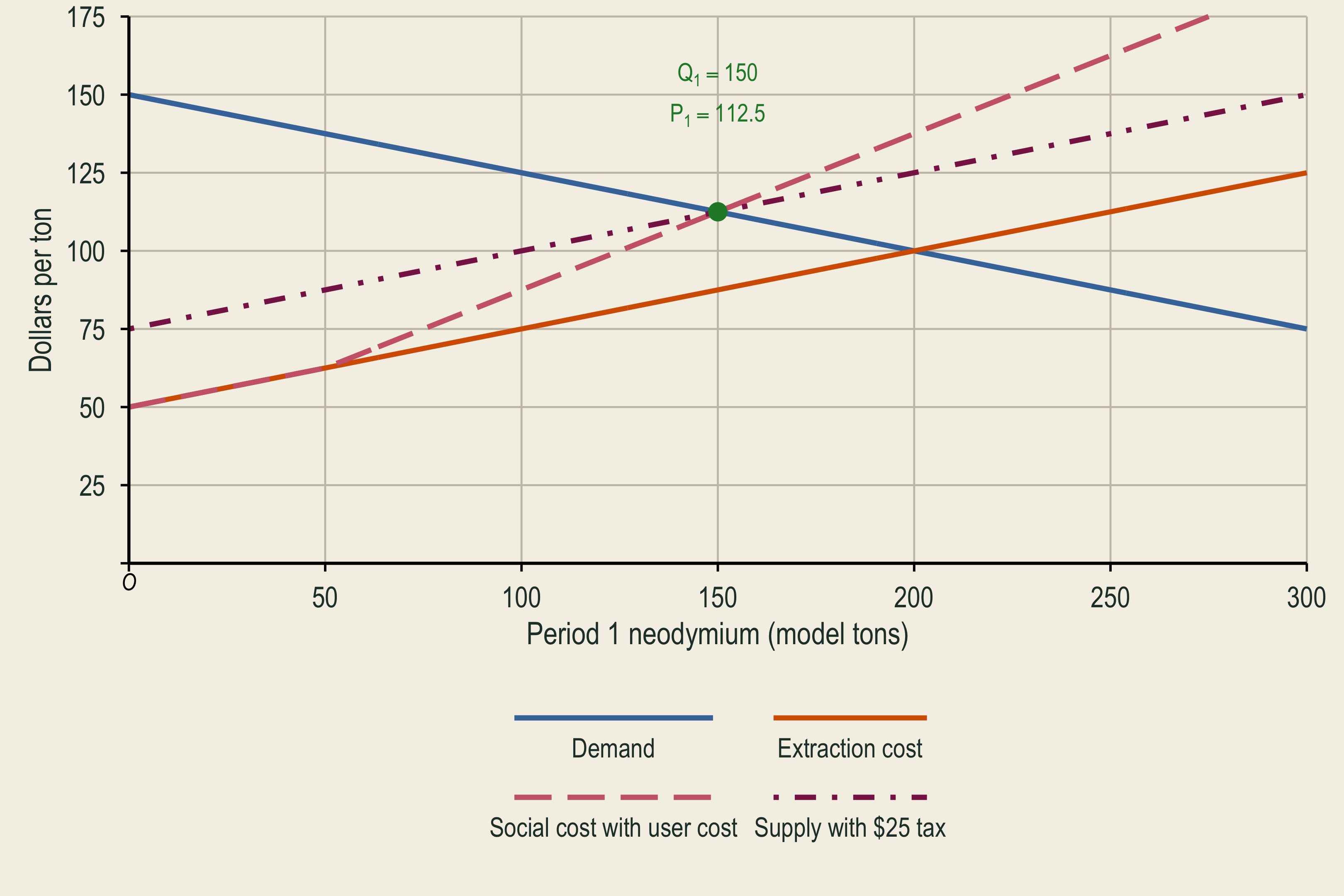
A resource depletion tax charges for the future opportunity lost through current extraction.

At the target quantity,

\[ \tau=25. \]

The tax-adjusted supply curve is

\[ P_S=75+0.25Q_1. \]

Equating demand and tax-adjusted supply gives

\[ Q_1=150,\qquad P_1=112.50. \]

📦 The Remaining Stock Sets Period 2 Quantity

A vertical remaining-stock line at 100 tons meets Period 2 demand at a price of 125 dollars. — Figure 10

🧰 Policy Options for Conserving More for Later

A depletion tax adds the future opportunity cost to the current extraction decision.

An extraction limit directly caps how much may be mined now, but it requires measurement and enforcement.
A reserve keeps selected deposits underground for future use.
A public stockpile buys and stores processed neodymium material for later release, but storage is costly.

Discussion: To leave more neodymium for Period 2, would you use a tax, a limit, or a reserve? Why?

📈 Scarcity Rent and Hotelling

💰 Scarcity Rent When 50 Tons Remain

Demand and marginal extraction cost are shown with a remaining-stock limit of 50 tons. At 50 tons, the market price is 137 dollars and 50 cents, marginal extraction cost is 62 dollars and 50 cents, and the vertical difference is scarcity rent of 75 dollars per ton. — Figure 11

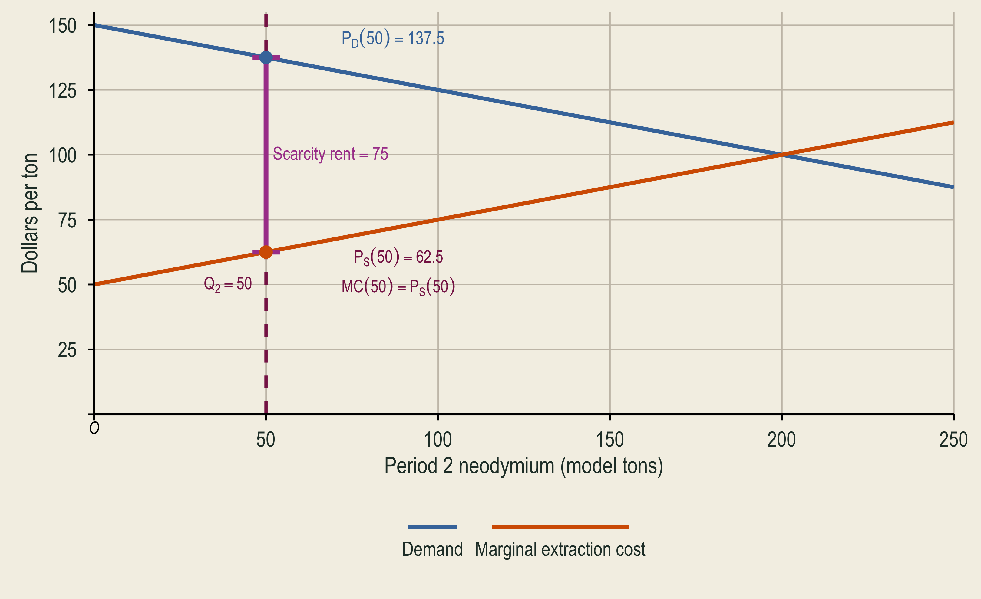
The stock limit fixes $Q_2=50$. The market price covers $62.50 of extraction cost plus $75 of scarcity rent, the value of using one unit of the limited stock.

🏦 A Forward-Looking Owner May Conserve

An owner compares small current profits with potentially larger future scarcity rent.

Leaving neodymium in the deposit can be profitable when its discounted future rent exceeds today’s rent.

Under strong assumptions, private owners can produce the same allocation as the depletion tax.

Policy remains relevant when owners do not foresee scarcity, cannot secure future value, or face incentives that differ from social welfare.

Discussion: When would a private owner’s timing decision also maximize social welfare?

📉 Discount Rates Change the Allocation

A fan of discounted Period 2 marginal net benefit curves moves lower as the discount rate rises, shifting the efficient crossing toward more Period 1 use. — Figure 12

📋 Discount Rates Shift Use Earlier

Annual rateApprox. ten-year factor$Q_1$$Q_2$

Annual rate	Approx. ten-year factor	$Q_1$	$Q_2$
0%	1.0	125	125
2%	1.2	132	118
5%	1.6	143	107
7.5%	2.0	150	100
10%	2.6	158	92
15%	4.0	170	80
20%	6.2	179	71
30%	13.8	190	60

Higher rates give Period 2 less present weight and shift the efficient allocation toward Period 1.

📈 Hotelling’s Rule

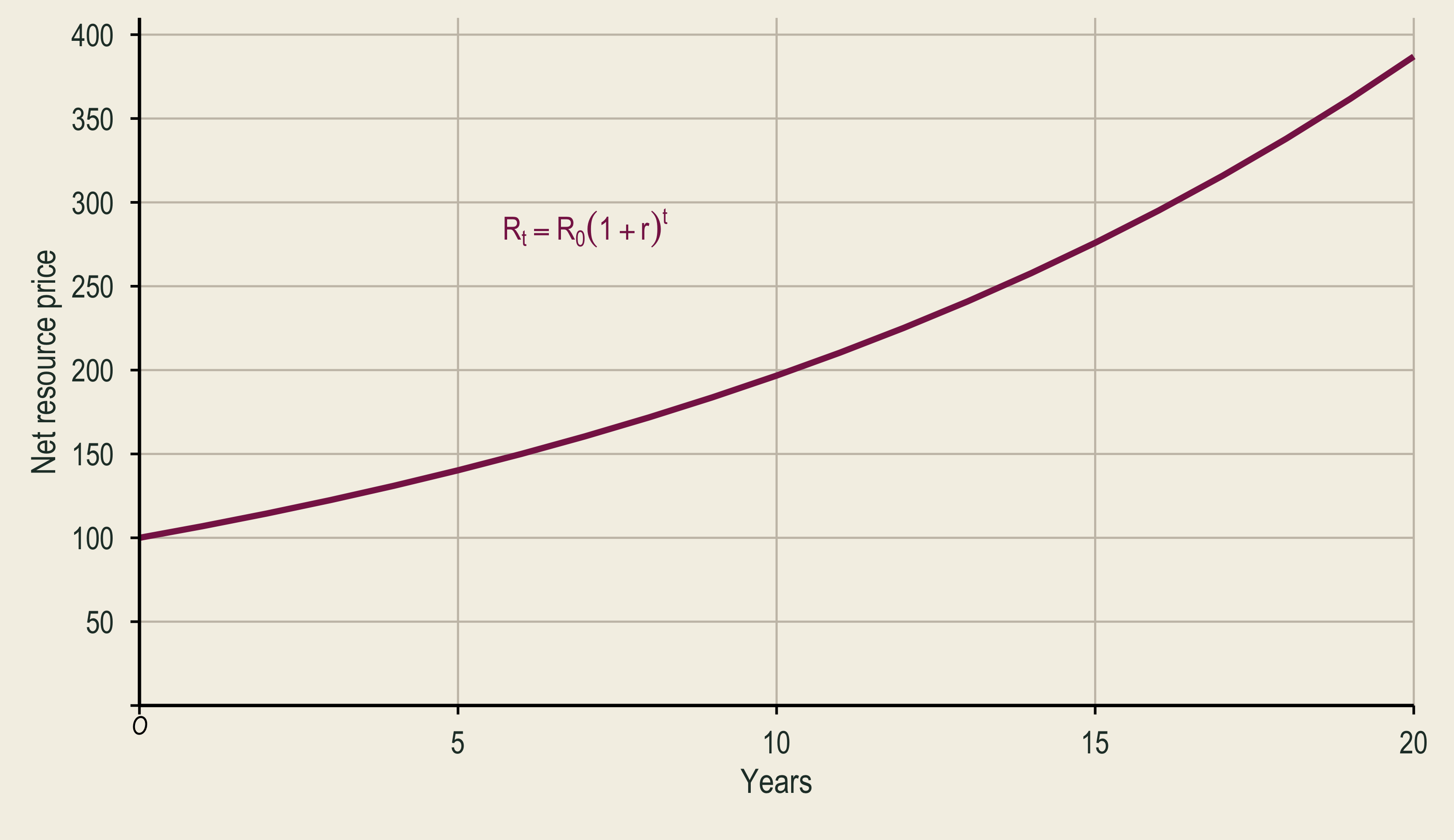
Hotelling’s rule states that the net resource price rises at the market interest rate in equilibrium.

Let

\[ R_t=P_t-MC_t. \]

Then the benchmark condition is

\[ R_{t+1}=(1+r)R_t. \]

⚖️ The Owner’s Timing Choice

Extract now when today’s rent invested at interest exceeds expected future rent.
Wait when expected future rent exceeds today’s rent plus interest.
Supply adjusts until the two choices have the same value at the margin.

The rule is an arbitrage condition for leaving the resource underground.

📈 The Benchmark Net-Price Path

Net resource price rises exponentially from 100 over 20 years at a 7 percent interest rate. — Figure 13

⛏️ The Optimal Depletion Rate

The optimal depletion rate maximizes the resource’s net present value.

Higher interest rates make earlier extraction more attractive.

Lower rates give stronger incentives to conserve.

Under the benchmark assumptions, complete exhaustion can be economically optimal.

Discussion: What should current users leave behind?

🏗️ Using Scarcity Rent for the Future

Hotelling asks when to extract. Hartwick asks how to use scarcity rent.

Invest scarcity rent rather than consume it.

Under the model’s assumptions, reinvesting the rent can replace lost natural wealth and help sustain consumption over time.

The rule does not preserve the neodymium deposit. It seeks to preserve the economy’s capacity to support future well-being.

This requires other forms of capital to replace the value lost through depletion. The assumption is more plausible for mineral deposits than for critical ecosystems with irreplaceable functions.

🕰️ Discounting and Distant Generations

Commercial interest rates can place very little present weight on effects far in the future.

A positive rate therefore shifts resource use toward earlier generations.

The remaining question is normative as well as financial:

Should a market return determine how society values distant generations?

🔎 Empirical Evidence on Hotelling’s Rule

What is tested: scarcity rent—not the raw market price—should rise at the interest rate, but extraction-cost and rent data are difficult to observe.
Observed paths: from 1970 to 2004, prices of 13 of 14 minerals had approximately zero long-run growth (Lin & Wagner, 2007).
Slade (1982): relative prices often followed a U-shaped path as technological progress dominated early and depletion pressures strengthened later.
Why paths differ: exploration, discovery, ore quality, technology, investment, recycling, market power, and policy all affect observed prices.
Takeaway: Hotelling’s rule is a benchmark for organizing these forces, not a literal price forecast.