Lecture 7

Valuing the Environment: Methods

Byeong-Hak Choe

SUNY Geneseo

🌿 Conservation Choices: Class Results

🌿 Our Conservation Choices

Trees, wildlife, and a stream represent the conservation supported by the choices.

22 participants made 264 decisions across twelve cards each.

69.7% of decisions selected a donation.

30.3% of decisions kept all cash.

What were you willing to give up for conservation?

💵 Same Gift, Different Cost

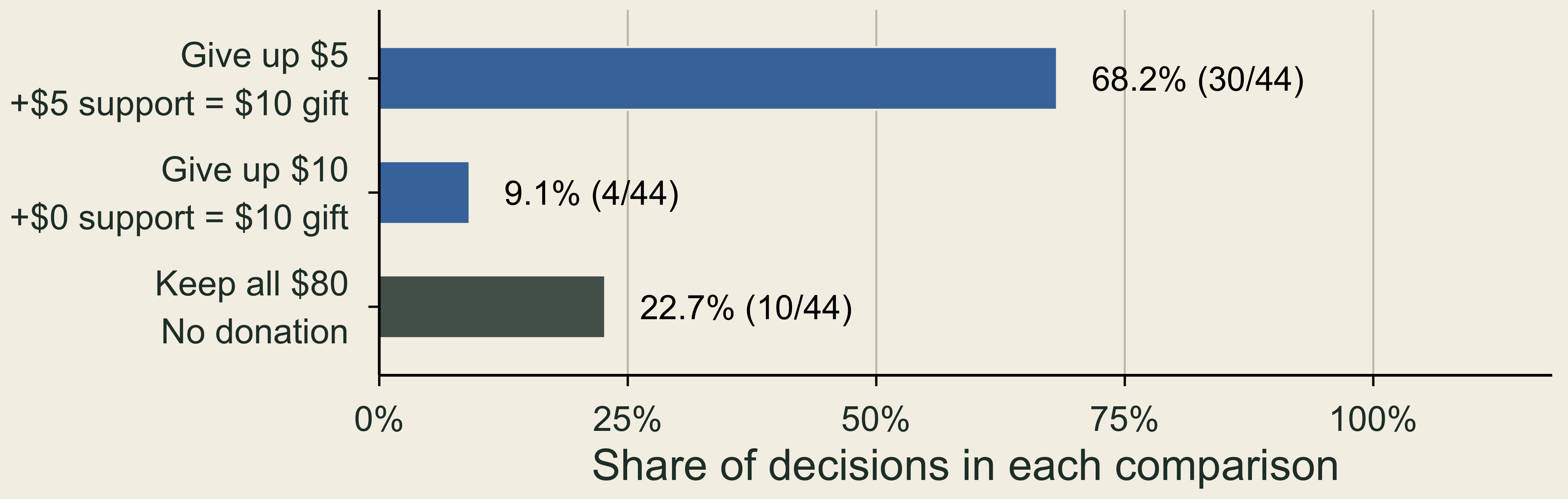
Both offers send $10 on the card to an organization. One asks for $5 from your cash, the other $10.

For the same displayed ten-dollar gift, 68.2 percent chose the five-dollar personal contribution, 9.1 percent the ten-dollar contribution, and 22.7 percent kept all cash.

Payment rule: actual amounts are 10% of card amounts. 44 decisions by 22 people.

🌱 Same Cost, Different Gift

Both offers ask for $15 from your cash on the card. Support increases the gift from $20 to $30.
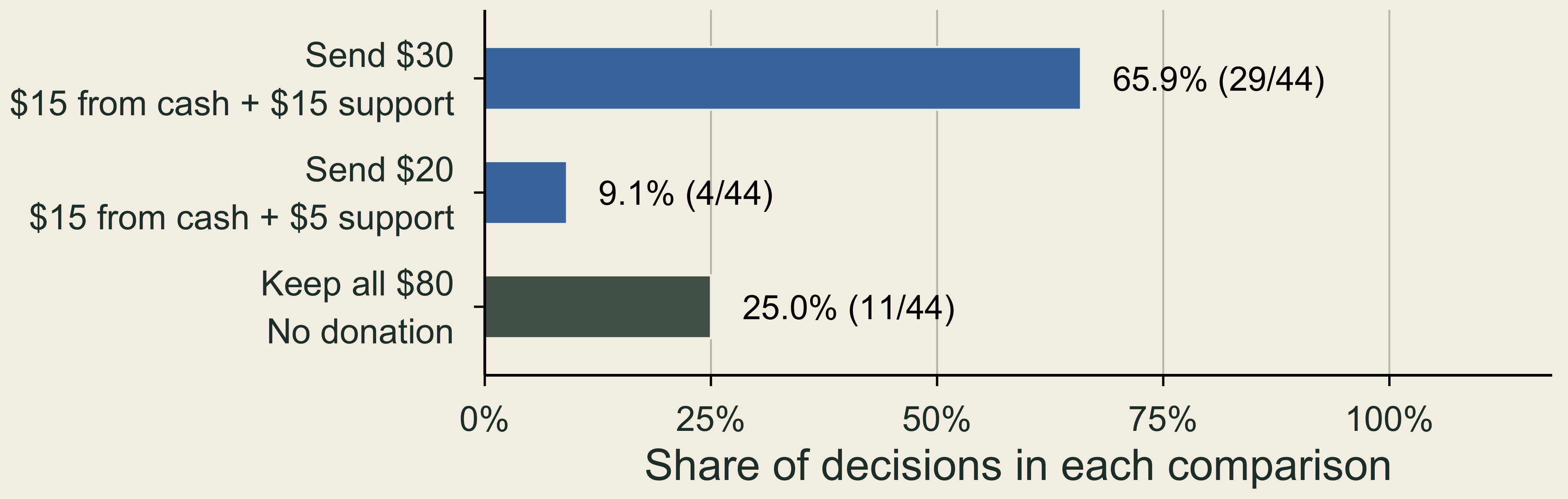
With the same displayed fifteen-dollar personal contribution, 65.9 percent chose the thirty-dollar gift, 9.1 percent the twenty-dollar gift, and 25 percent kept all cash.

Payment rule: actual amounts are 10% of card amounts. 44 decisions by 22 people.

📈 What the Regression Adds

Outcome on twelve cards: chosen = 1, otherwise 0. Relative chance: predicted chance of choosing the offer relative to that of keeping cash.
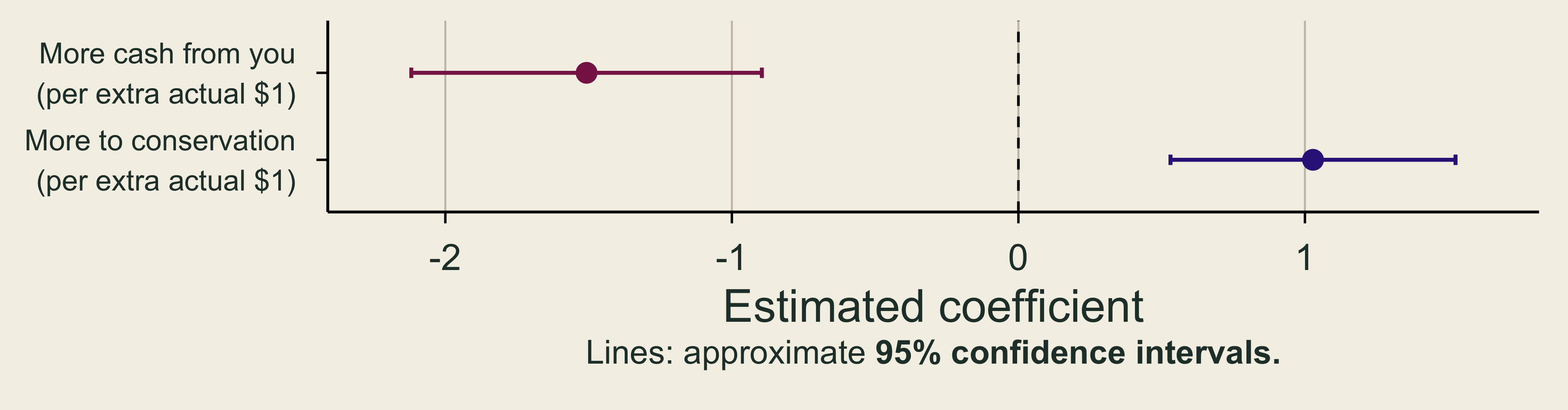
The personal-cost coefficient is negative and the delivered-gift coefficient is positive, with approximate 95 percent confidence intervals.

  • Cost coefficient (-1.507): An extra actual $1 from your cash lowers the offer’s relative chance by 78%, for the same gift \((1-\exp(-1.507)\approx 0.78)\).
  • Gift coefficient (1.028): An extra actual $1 to conservation raises the offer’s relative chance by 180%, for the same personal cost \((\exp(1.028)-1\approx 1.80)\).

💰 One Extra Dollar to Conservation

Marginal WTP (MWTP): the most extra cash you would give up for one more unit. Here, the unit is $1 more to the same organization.

  • Add $1 to an offer’s gift: its relative chance rises (coefficient +1.028).
  • Add $x to its cost to you: it falls (coefficient −1.507 per $1).

Break-even: MWTP is the x that leaves the relative chance unchanged. \[ 1.028-1.507\,x=0 \quad\Rightarrow\quad \text{MWTP}=x=\frac{1.028}{1.507} \approx\$0.68. \]

In our choices, $1 more for conservation was worth about 68¢ of our own cash (95% CI: $0.60–$0.76).

If that extra $1 costs you less than 68¢, the larger gift is more attractive; exactly 68¢, equally attractive; more than 68¢, less attractive.

🤝 Using MWTP: How Big Must a Match Be?

Real campaign (2025): to care for its Little Italy Nature Preserve, Genesee Valley Conservancy had gifts matched $1 for $1, up to $200,000.

Match m per $1 Your cost: $1 ÷ (1 + m) Below 68¢?
None $1.00 No
25¢ 80¢ No
50¢ 67¢ Yes, barely
75¢ 57¢ Yes
$1 (actual) 50¢ Yes

Smallest match that makes a larger gift more attractive: about 47¢ per $1.

Why not always match generously? The foundation’s $200,000 runs out:

  • at $1 per $1, after donors give $200,000;
  • at 50¢ per $1, after donors give $400,000.

Implication: $1 per $1 is more than needed. If donors would give over $200,000, a 75¢ match would still work and stretch the $200,000 further.

🌳 What Does This Reveal About Nature?

  • Opportunity cost: each dollar from your own cash is a dollar you could otherwise keep.
  • Choices reveal how much people will give up: our offers let us estimate a trade-off between personal cash and conservation funding.
  • For a policy, define the improvement: cleaner water or protected habitat relative to a clear baseline, then compare its benefits with costs.

Cleaner water and protected habitat often have no posted price. How can we measure these benefits when a market price does not record them?

🌿 Environmental Value and Willingness to Pay

🌊 Oil Spills and Environmental Losses

Spills harm fishing, recreation, wildlife, and habitats.

Spill Environmental valuation Civil settlement
Exxon Valdez About $2.8 billion
(1990 dollars)
$900 million
(1991)
Deepwater Horizon At least $17.2 billion
(2017 study)
$20.8 billion
(2016)
  • Surveys include the value of wildlife and habitat even to people who never visit.
  • Settlement payments are not survey estimates of damages.

Does paying for cleanup compensate people for everything they lost?

⚖️ Why Put Environmental Benefits in the Comparison?

  • Benefit–cost analysis: compare environmental gains with resources used to obtain them.
  • Damage assessment: identify lost services and guide restoration or compensation.
  • Leaving a benefit unmeasured does not make it zero.

If an analyst counts the cost of protecting a wetland but omits its benefits, which choice will look more attractive?

🔬 From Environmental Change to Welfare

Step A cleaner-river example
1. Define the baseline Which change and which people?
2. Estimate physical effects Fewer illnesses and healthier fish
3. Account for responses Less filtering water or avoiding swimming
4. Value the consequences Avoided costs and remaining welfare gains

Check: could income, age, or another change explain the observed difference?

🦆 Use, Option, and Nonuse Values

1. Use 2. Option 3. Nonuse
Value from using a resource or benefiting from the services it provides. Value from keeping future personal use possible when that use is uncertain. Value from a resource's existence or preservation for others, without personal use.
Examples: fishing, birdwatching, or flood protection. Example: keeping the option to visit a forest later. Examples: species survival and preserving nature for future generations.

\[\text{Total WTP}=\text{use}+\text{option}+\text{nonuse values}.\]

📈 Marginal WTP and the Value of an Improvement
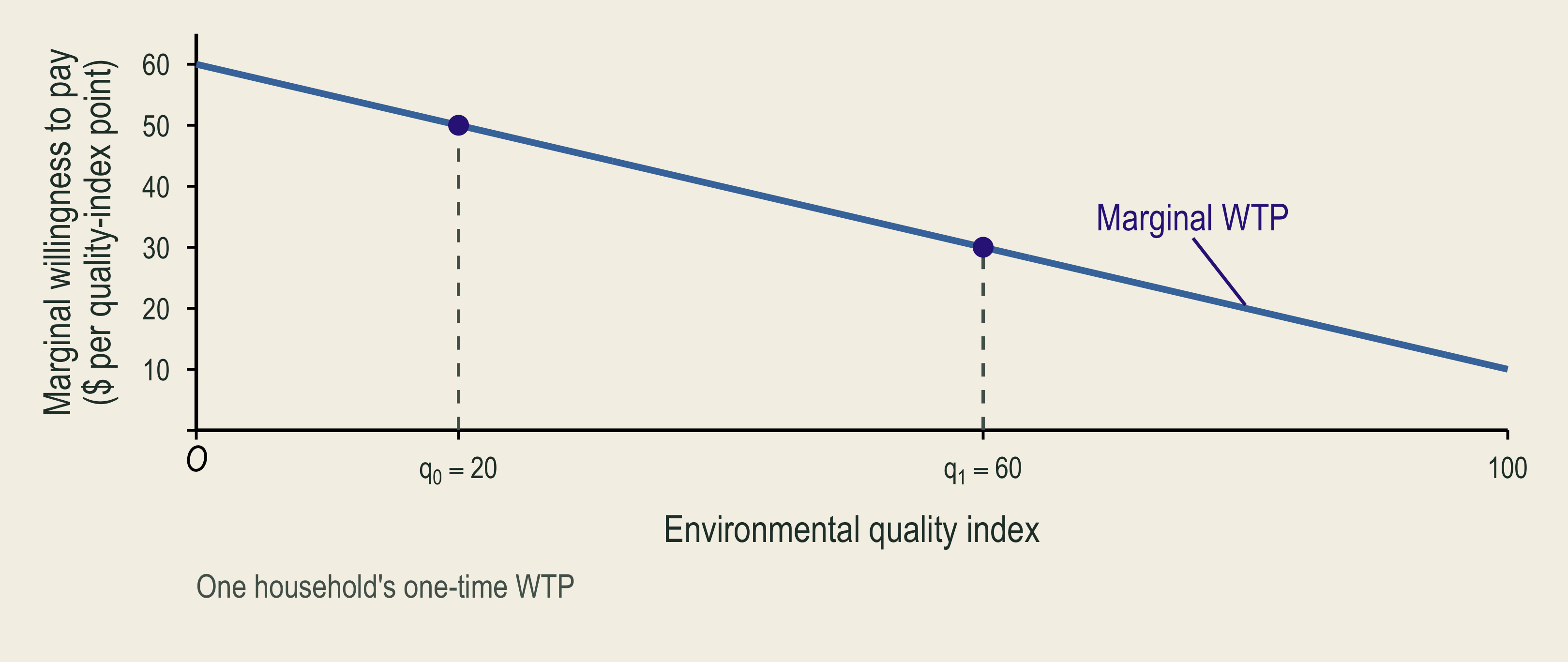
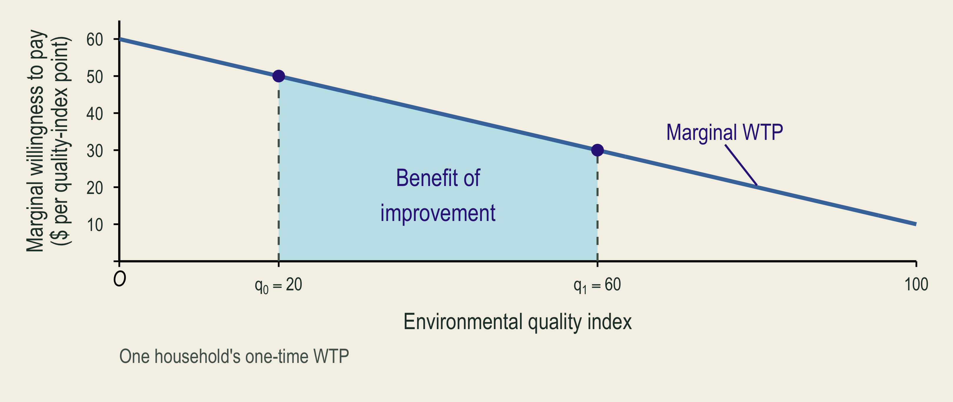
One household's marginal willingness to pay declines as environmental quality improves.

The area under marginal willingness to pay between the baseline and the improved quality measures the household's benefit.

  • MWTP (marginal willingness to pay): the most a household would pay for one more unit of environmental quality.
  • The area under MWTP over the improvement gives total WTP for that change.

💵 Willingness to Pay and Willingness to Accept
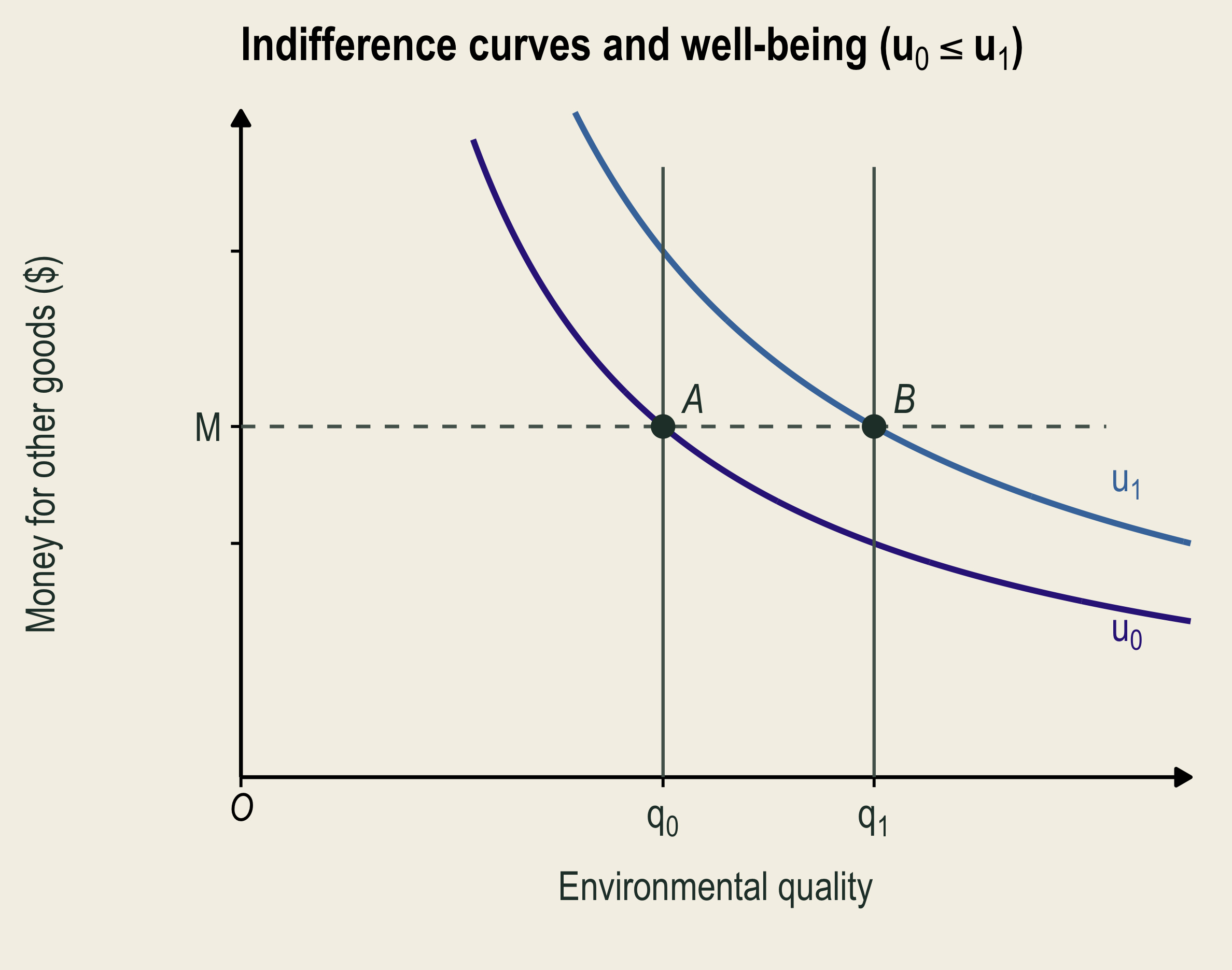
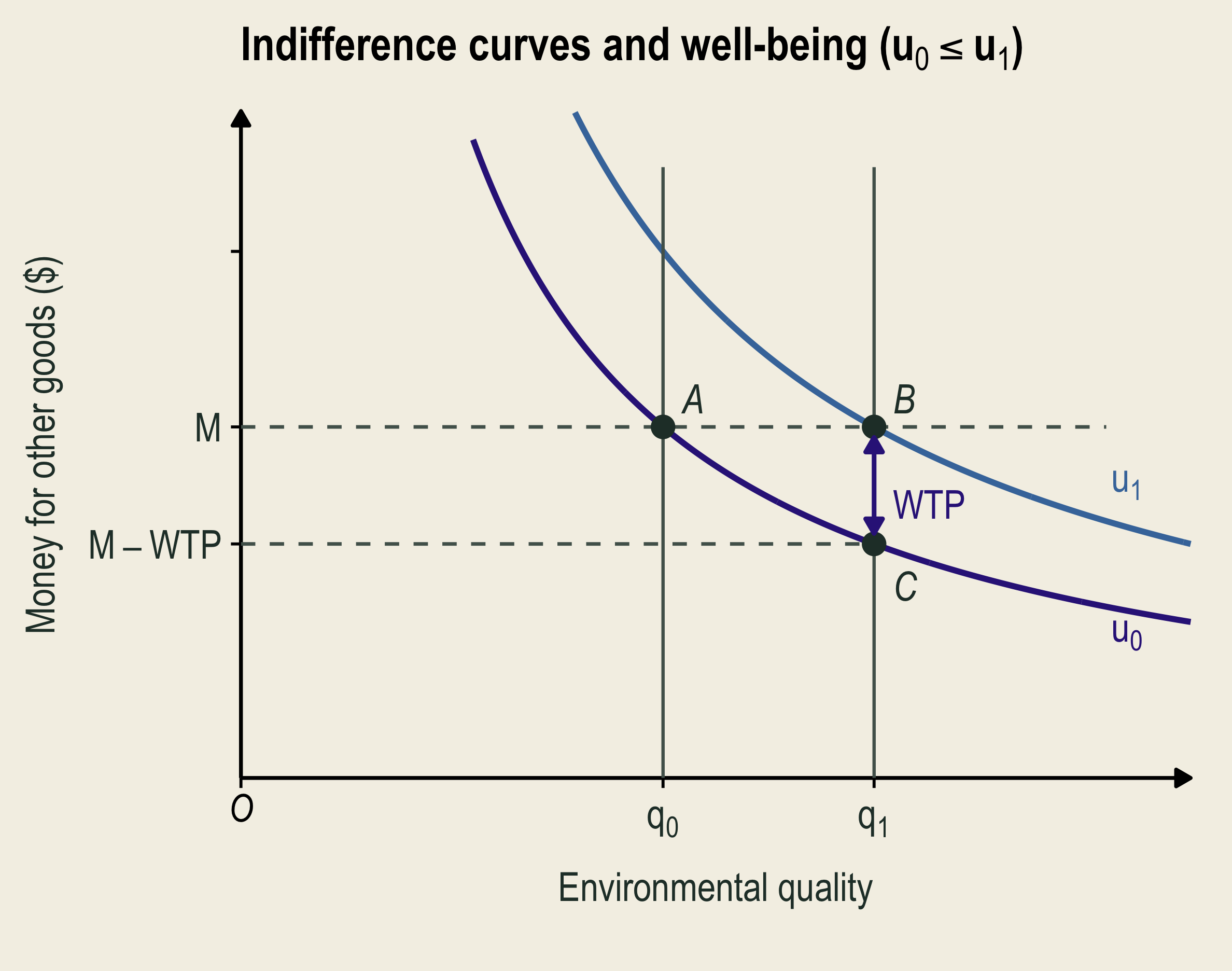
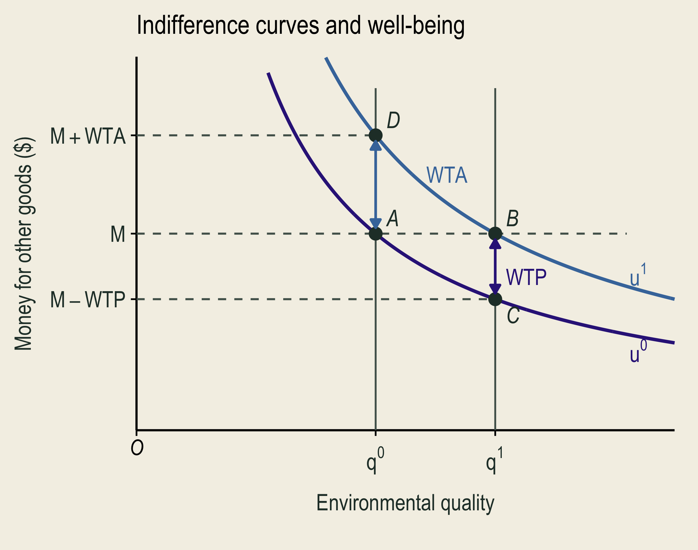
At the same money M, A has original environmental quality and well-being u-zero; B has improved quality and well-being u-one. Black axis arrowheads mark increasing environmental quality and money for other goods.

A to B is the environmental improvement. A two-headed vertical segment between B and C measures WTP. Paying this amount leaves C at the same original well-being as A.

A two-headed vertical segment between A and D measures the least compensation accepted for the degradation, restoring well-being u-one. WTA appears to the left of this segment.

At money \(M\), A to B is an improvement; B to A is a loss.

Willingness to pay (WTP) is the most someone would pay for an environmental improvement.

Paying \(\,\overline{\;BC\!}\;\,\) leaves you as well off as at A (\(\color{#332288}{u_0}\)).

Willingness to accept (WTA) is the least compensation someone would accept for an environmental loss.

Receiving \(\,\overline{\;AD\!}\;\,\) leaves you as well off as at B (\(\color{#4477AA}{u_1}\)).

🌳 WTP and WTA: Four Park Scenarios

Situation Valuation question Measure
A park could be expanded. Most you would pay for the expansion? WTP
An existing park could shrink. Most you would pay to prevent the loss? WTP
An existing park could shrink. Least compensation you would accept for the loss? WTA
A promised expansion could be canceled. Least compensation you would accept instead of the expansion? WTA

WTP can measure avoiding a loss; WTA can measure forgoing an improvement.

The entitlement (starting right) helps identify whether to ask about paying or receiving compensation.

🌳 WTA–WTP Differences: Limited Substitutes
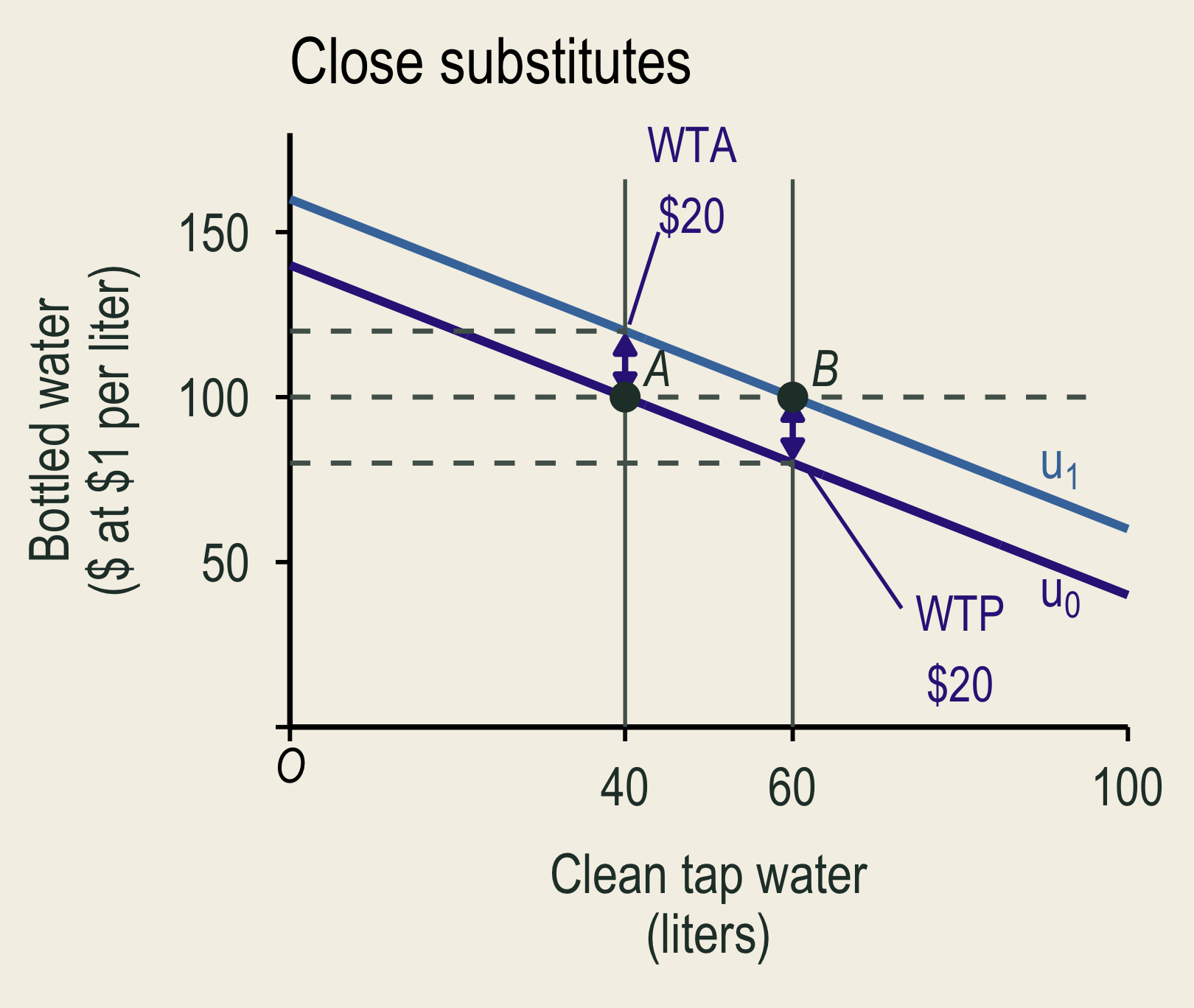
Clean tap water and equally safe bottled water are close substitutes. WTA and WTP for twenty more liters of tap water both equal twenty dollars.

Equally safe bottled water costs $1 per liter. Here, WTA = WTP = $20.
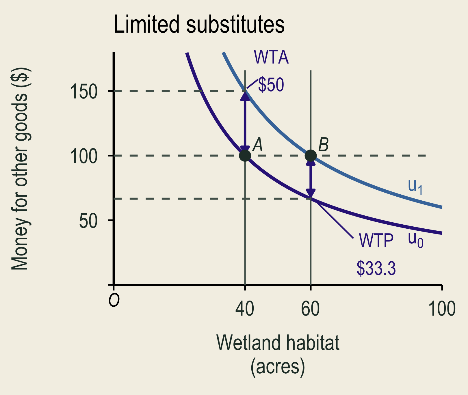
Wetland habitat and money for other goods are limited substitutes. WTA is fifty dollars, while WTP is about thirty-three dollars.

Money may not replace lost wetland habitat. WTA can exceed WTP.

📉 WTA–WTP Differences: Gains and Losses Can Feel Different
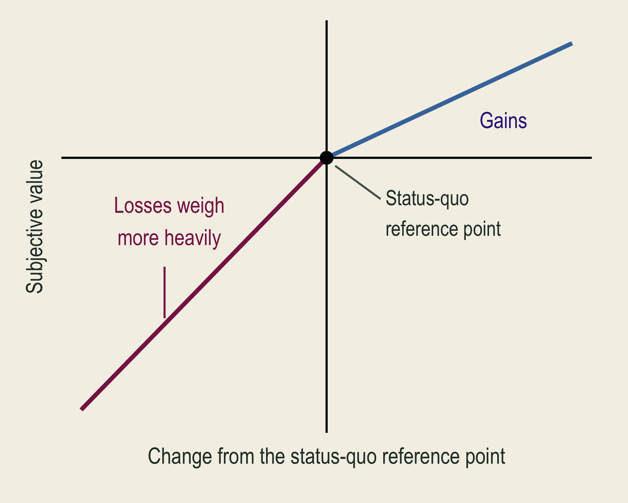
An S-shaped well-being curve shows a larger loss than gain for equal changes in environmental quality around the status quo. A black upward arrow denotes increasing utility or well-being, and a black rightward arrow denotes increasing environmental quality. A colored left-pointing arrow identifies WTA as minimum compensation to accept the loss; a colored right-pointing arrow identifies WTP as maximum payment to obtain the gain.

Prospect theory: people value gains and losses differently.

  • Reference point (status quo): the environmental quality you currently enjoy.
  • Loss aversion: an equal-sized quality loss can hurt more than the gain feels good.
  • Endowment effect: people may ask for more to give up an amenity (WTA) than they would pay to obtain it (WTP).

🌳 Why WTA and WTP Can Differ

  1. Limited substitutes
  2. Loss aversion and the endowment effect
  3. Income: a limited budget can constrain WTP.
    • A tight budget limits WTP to save a park, but does not cap compensation requested for losing existing access.
  4. Uncertainty and commitment costs: deciding now can mean giving up the chance to wait for more information.
    • Damaged well: if a final settlement rules out later claims, a household may ask for more compensation while health risks are uncertain.

🌍 Valuation and Other Decision Criteria

What dollar totals can miss Why valuation still helps
Income: low WTP can reflect a tight budget. Protection uses scarce resources.
Distribution: net gains do not guarantee compensation for those who lose. Unmeasured benefits should not count as zero.
  • Compare monetary estimates alongside rights and ecological limits.

Two wetland plans have similar measured net benefits. One also protects habitat with unmeasured value.

What would you check about the habitat and the people affected before choosing?

🔎 Two Sources of Valuation Evidence

Revealed preference

  • Observed choices in related markets.
  • Trips, housing, jobs, and protective purchases.
  • Usually captures values linked to behavior.

Stated preference

  • Choices about a described environmental change.
  • Contingent valuation and choice experiments.
  • Can include values held by nonusers.

🗳️ Stated-Preference Methods

🗳️ Contingent Valuation: A Survey About a Change

Contingent valuation (CV) uses a survey to ask what people would pay for, or accept as compensation for, a described change.

  • A full survey describes the baseline, change, and payment, with valuation, follow-up, and background questions.
  • Valuation formats include yes/no questions, amounts, and follow-up bids.

Baseline: pollution closes a lake to swimming for 20 days each summer.

Would your household pay $30 per year for five years, through a local tax, for a program that prevents those closures?

  • Without the program, the closures continue. This question is one part of a full survey.

🧪 Survey Design: Information Bias

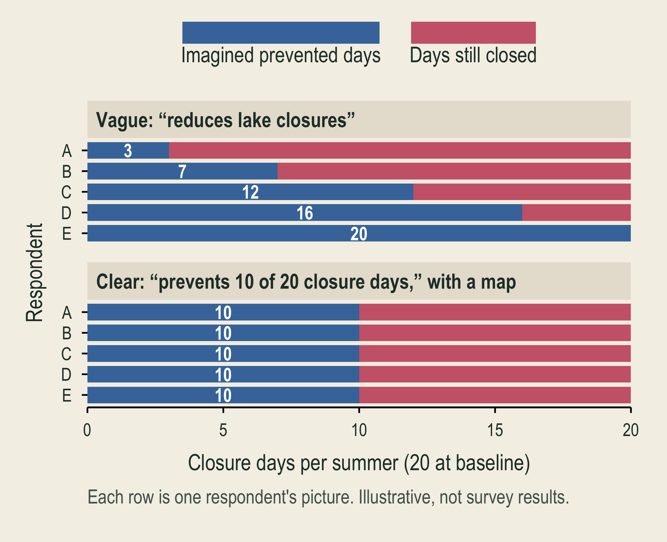
Bars show what five illustrative respondents picture when told about a program. After a vague description, they picture programs that prevent 3, 7, 12, 16, and 20 of the 20 closure days. After a clear description with a map, all five picture a program that prevents 10 of the 20 closure days.

What to consider: People imagine different improvements, so respondents answer different questions.

In the figure: Each row is one respondent’s picture. A clear description with a map makes the pictures match.

What helps: Neutral descriptions; a map showing exactly which part of the lake the program covers; comprehension checks

🧪 Survey Design: Framing Effects
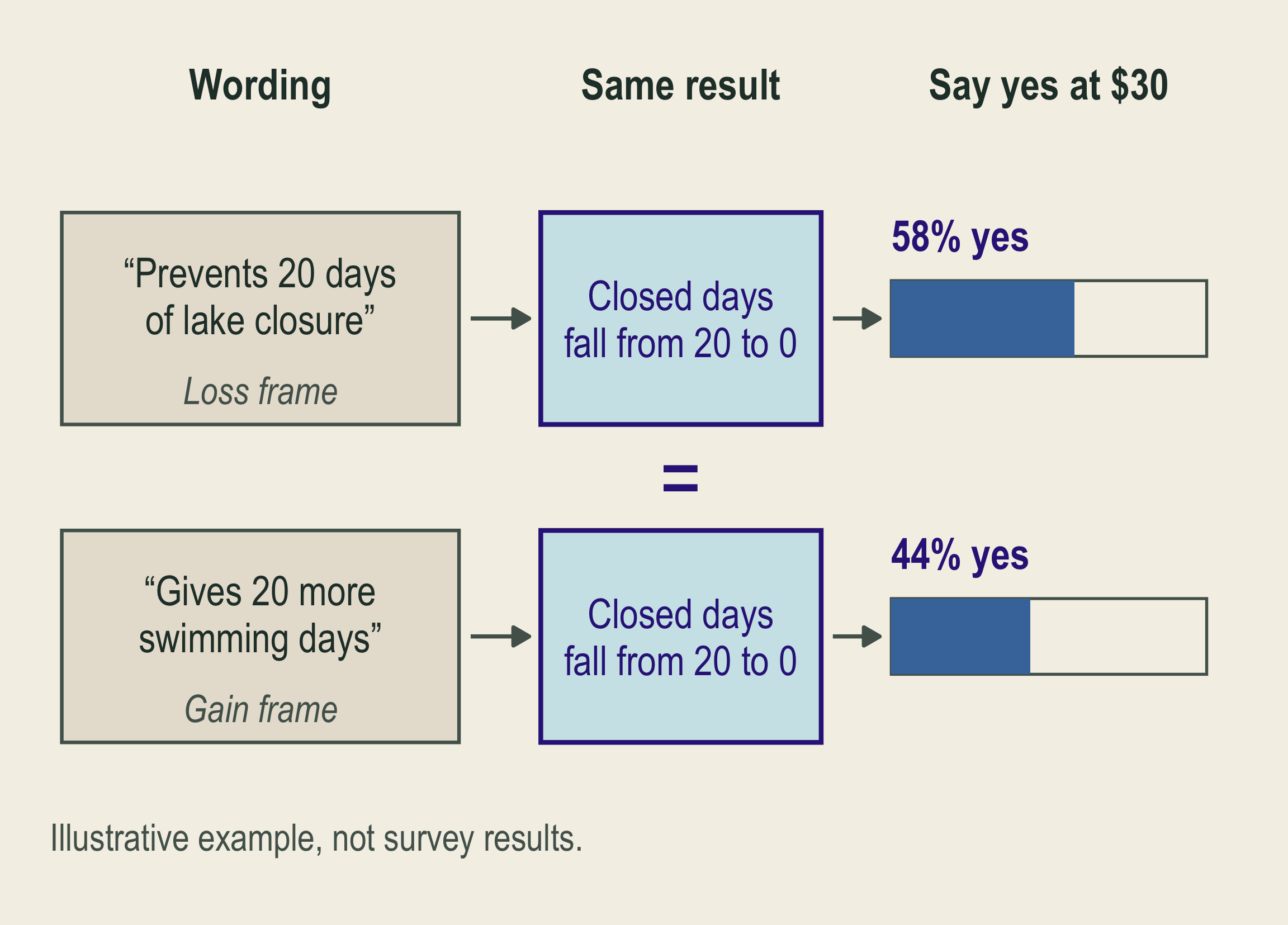
Two wordings of the same program result, closed lake days falling from 20 to 0, lead to different illustrative shares saying yes at 30 dollars: 58 percent for the loss frame 'prevents 20 days of lake closure' and 44 percent for the gain frame 'gives 20 more swimming days'.

What to consider: How the same program result is worded changes answers: a loss frame versus a gain frame.

In the figure: Both wordings describe the same result, yet the share saying yes at $30 differs.

What helps: Describe the same result in every wording (closed days fall from 20 to 0); test alternative wordings

🧪 Survey Design: Anchoring Effects
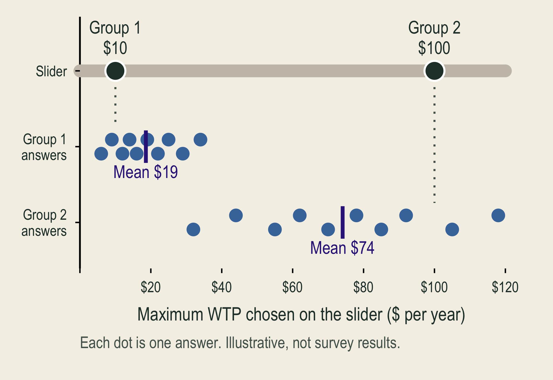
A dollar slider at the top starts at 10 dollars for Group 1 and at 100 dollars for Group 2. Below it, ten illustrative answers per group. Group 1 answers have a mean near 19 dollars. Group 2 answers have a mean near 74 dollars.

What to consider: A suggested $10 or $100 shapes later WTP. The starting amount is the first number respondents see.

In the figure: Respondents drag the slider to their maximum yearly payment. Each group’s answers stay near its starting amount.

What helps: Vary starting amounts; compare later answers

Only the starting amount differs, so a gap in answers points to it.

🧪 Survey Design: WTP–WTA Discrepancy
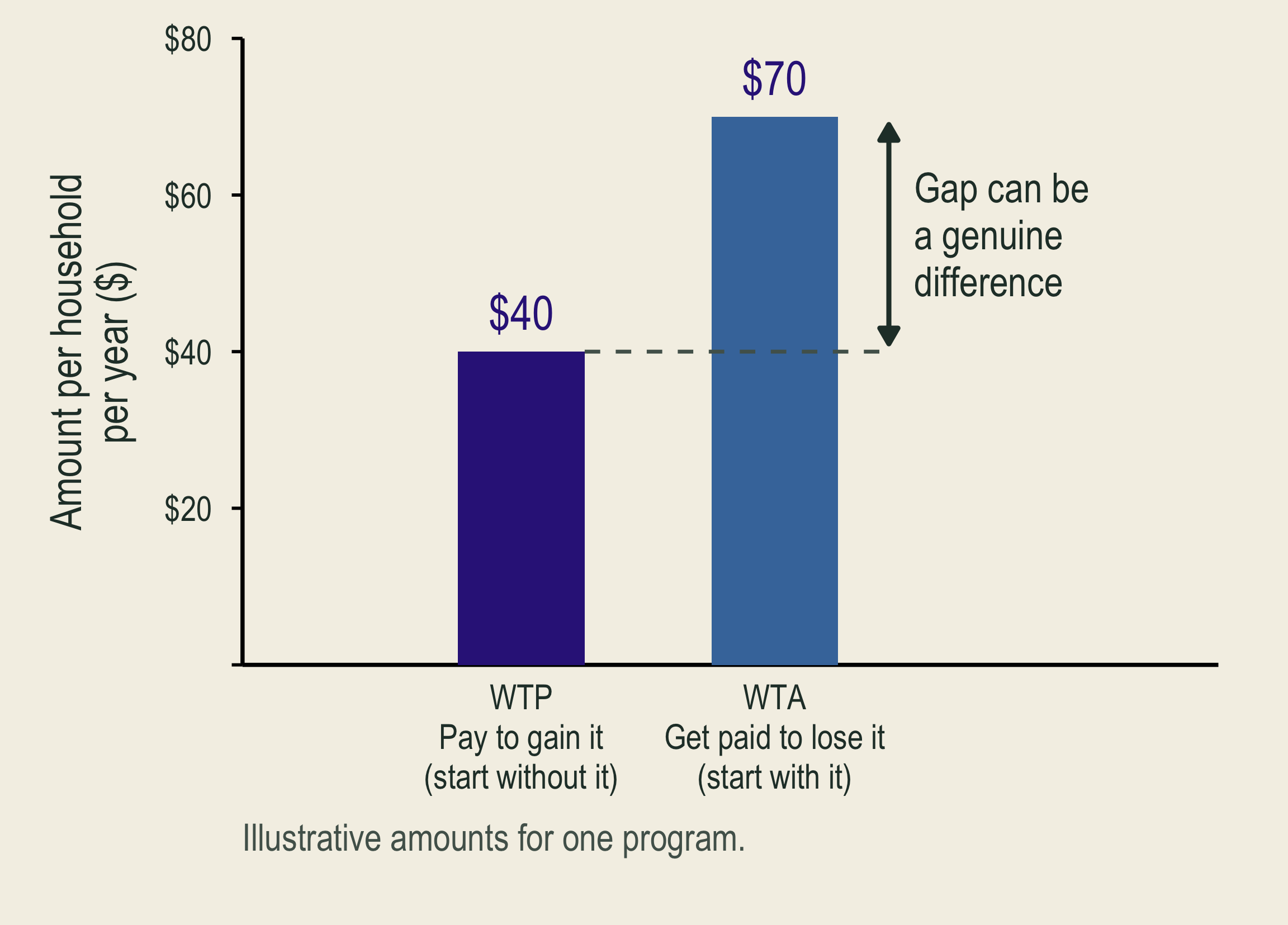
Bars show illustrative willingness to pay of 40 dollars and willingness to accept of 70 dollars for the same program. The gap can be a genuine difference because the starting rights differ.

What to consider: WTA can exceed WTP without bias. Limited substitutes, income, and reference points can make it larger.

In the figure: The same program, two questions: pay to gain it (WTP) or accept money to give it up (WTA).

What helps: Specify the change and starting rights; choose WTP or WTA.

💳 Survey Design: Strategic Answers
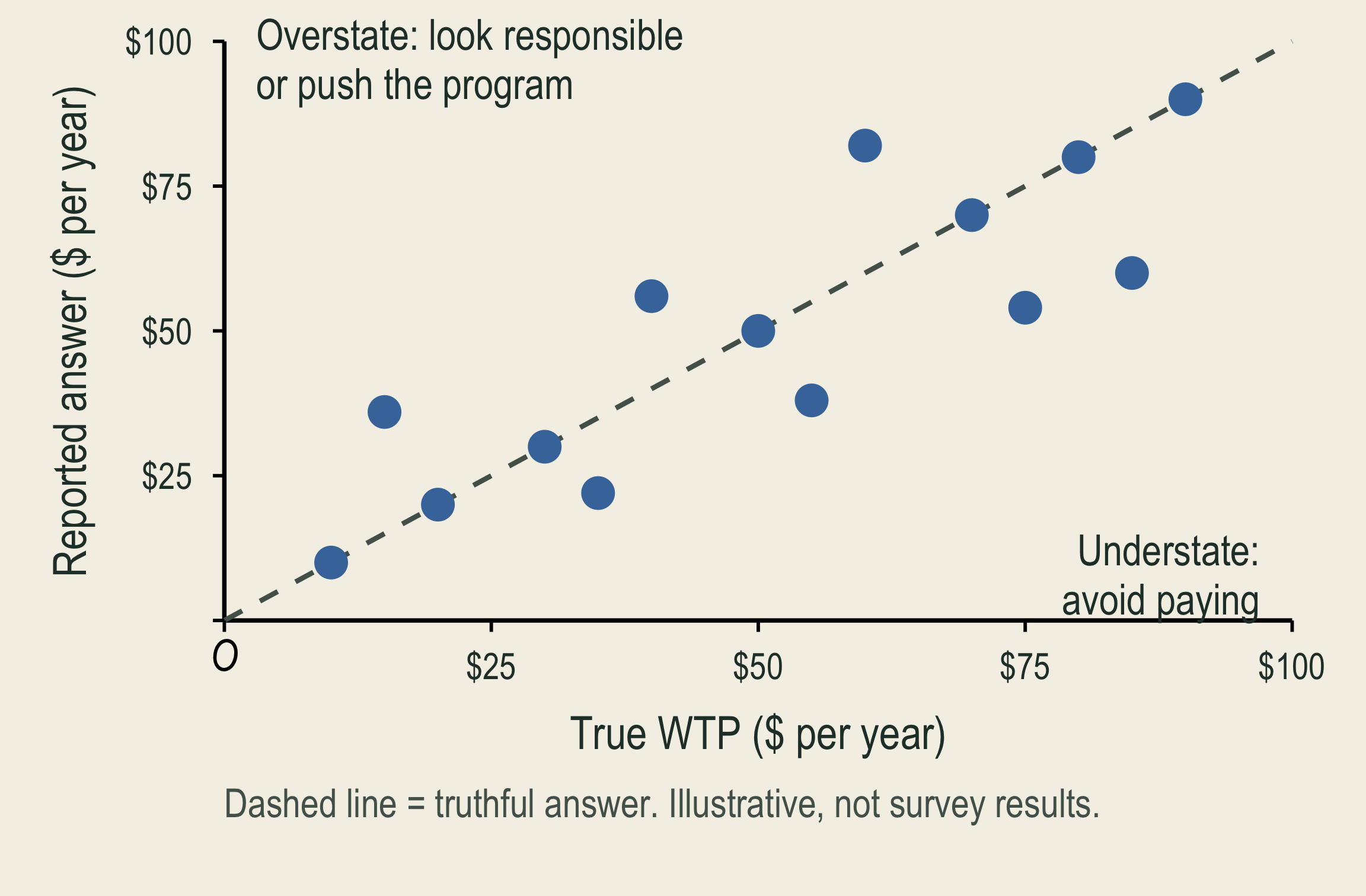
Illustrative reported answers plotted against true willingness to pay. Truthful answers lie on a dashed line. Some respondents report more than their true value, to look responsible or push the program. Others report less, to avoid paying.

What can go wrong: Misstate support to influence policy (strategic) or to look responsible (social desirability).

In the figure: Truthful answers lie on the dashed line. Dots above it overstate; dots below it understate.

What helps: Private answers; a clear decision rule (votes decide whether the program goes ahead) and payment rule (everyone pays the same stated price)

Then understating cannot lower your bill; a yes accepts the price.

💳 Survey Design: Hypothetical Bias
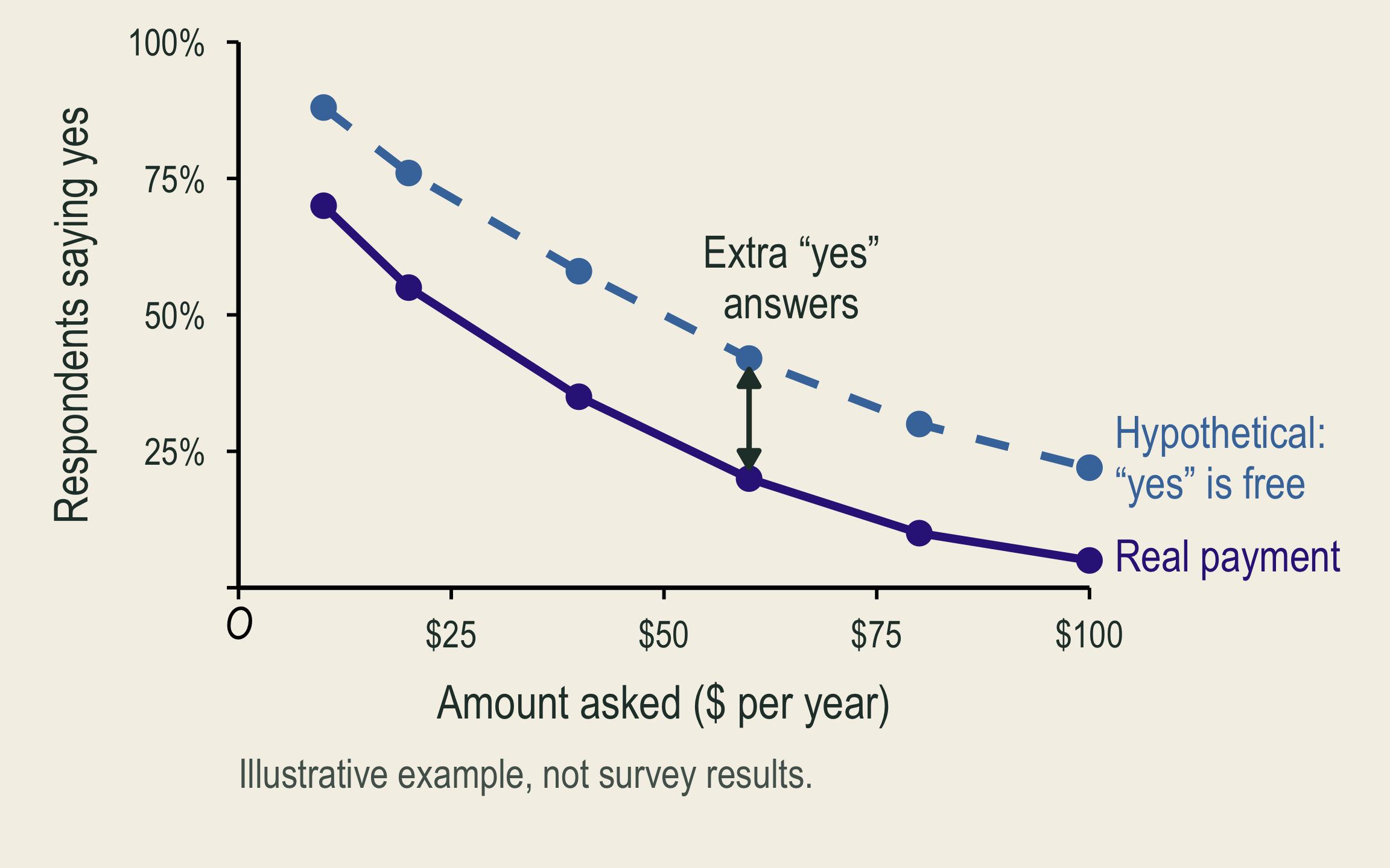
Illustrative share saying yes falls as the amount asked rises under both questions, but the hypothetical question yields a higher share than real payment at every amount.

What can go wrong: “Yes” feels costless without real payment.

In the figure: At every amount, more people say yes to the hypothetical question than when payment is real.

What helps: A budget reminder before the question, such as “think about what else this money would pay for”; credible consequences

Credible consequences: you believe choices can have real effects.

e.g., Nature, Your Choice: if your code and card are drawn, your chosen cash and donation are paid.

💳 Survey Design: Payment-Vehicle Effects
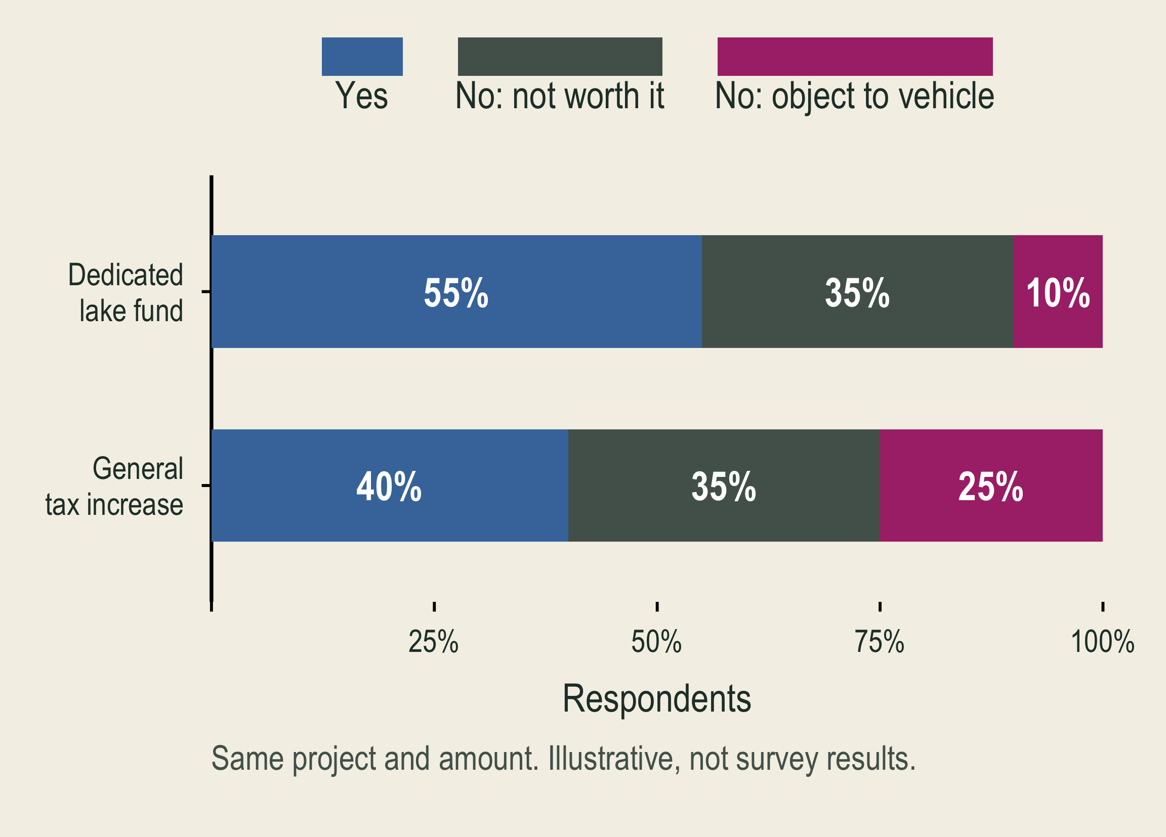
Stacked bars of illustrative responses to the same project and amount. A dedicated lake fund gets 55 percent yes, 35 percent no because the project is not worth it, and 10 percent no because respondents object to the vehicle. A general tax increase gets 40, 35, and 25 percent.

What can go wrong: Reject the tax or agency, not the project.

In the figure: “No: not worth it” stays at 35%, but “No: object to vehicle” rises from 10% to 25%.

What helps: Name the payment method the program would really use; ask about objections; test a different method

Follow-up questions separate a protest from a genuine zero WTP.

🧪 Survey Design: Embedding Bias
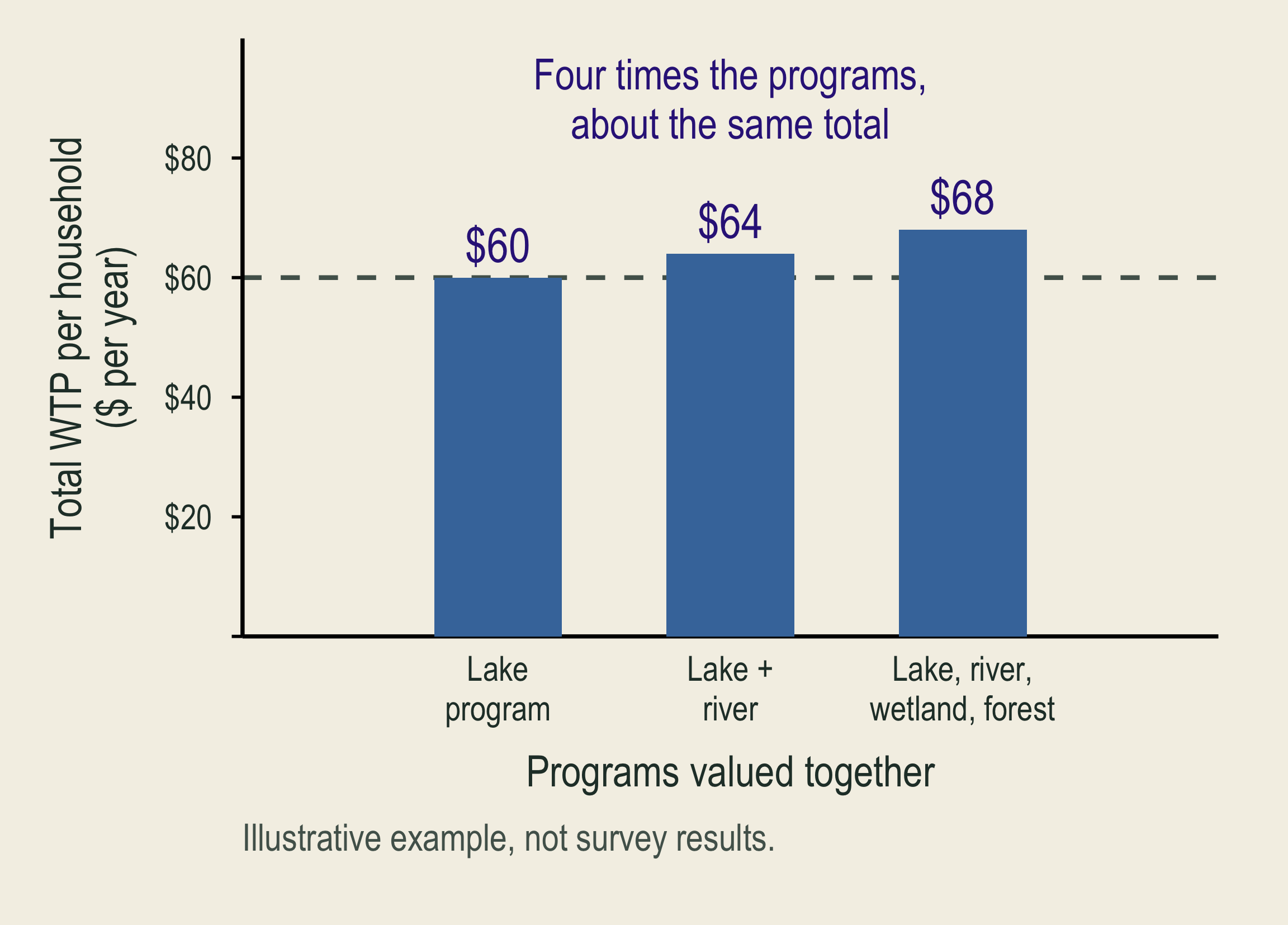
Bars show illustrative total willingness to pay when one, two, or four programs are valued together: 60, 64, and 68 dollars. Four times as many programs raises the total only slightly.

What to consider: A good’s stated value depends on what else is valued with it. Respondents struggle to separate it from related goods.

In the figure: Total WTP barely rises from one program to four: a warning sign, not proof.

What helps: Define exactly what is valued; compare the good alone, in a package, and after others

📏 Does a Bigger Improvement Raise WTP?

Same lake and population; baseline: 20 closure days each summer.
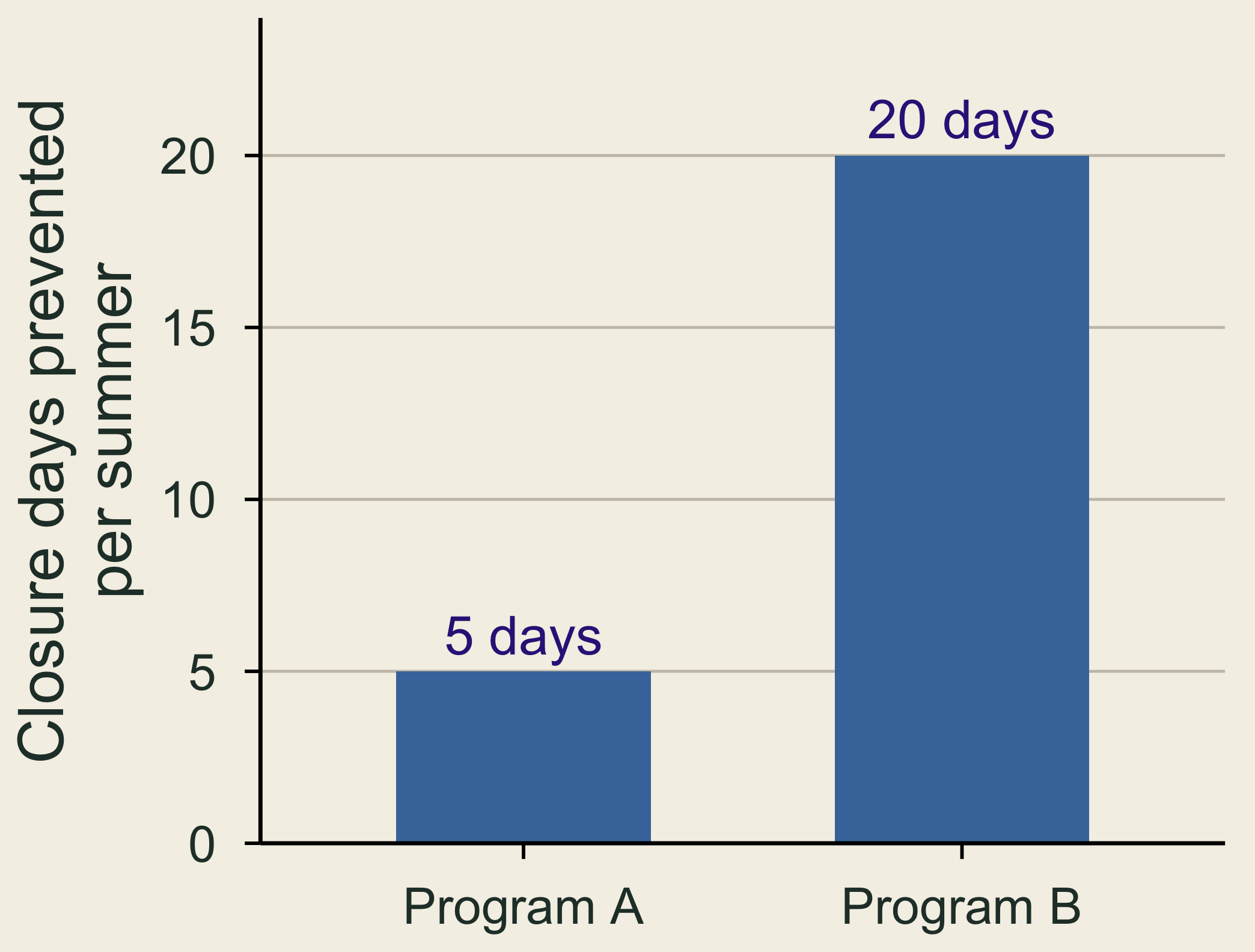
Two proposed programs prevent five versus twenty swimming-closure days per summer. The bars show the environmental changes, not willingness-to-pay estimates.

Days prevented, not WTP.

  • Scope test: compare WTP for A versus B, keeping the five-year tax rule fixed.
  • Warning sign: similar WTP for A and B, possibly from embedding or misunderstanding.
  • Check: ask respondents what change they imagined and why they chose the amount.

Interpretation: WTP need not quadruple, but similar WTP is a warning sign, not proof: small extra benefits or a tight budget can also explain it.

❔ A Zero Answer Can Have Different Meanings

“The improvement is not worth a payment to me.”

  • This may be genuine zero WTP, including a budget constraint.

“I care about the lake, but do not trust this payment scheme.”

  • This may be a protest response.
  • Use follow-up evidence. Do not automatically discard zeros.

🚢 Exxon Valdez: Survey Value and Settlement

  • A national survey offered an escort-ship program to prevent another spill.
  • Households chose yes or no at an assigned one-time tax.
Figure What it represents
About $2.8 billion
1990 dollars
Conservative estimate of nonuse values
$900 million
1991 agreement
Civil settlement for restoration and damages
  • The survey valued nonuse losses, including wildlife and habitat valued by people who never visit.

🐻 A Choice About Brown-Bear Protection

Bear-cam viewers watch live online video of brown bears fishing at Katmai National Park, Alaska.

Hypothetical proposal: viewers would donate to a bear-protection trust fund.

  • It would fund collision prevention, anti-poaching enforcement, and research, expected to prevent one bear death per year, on average.
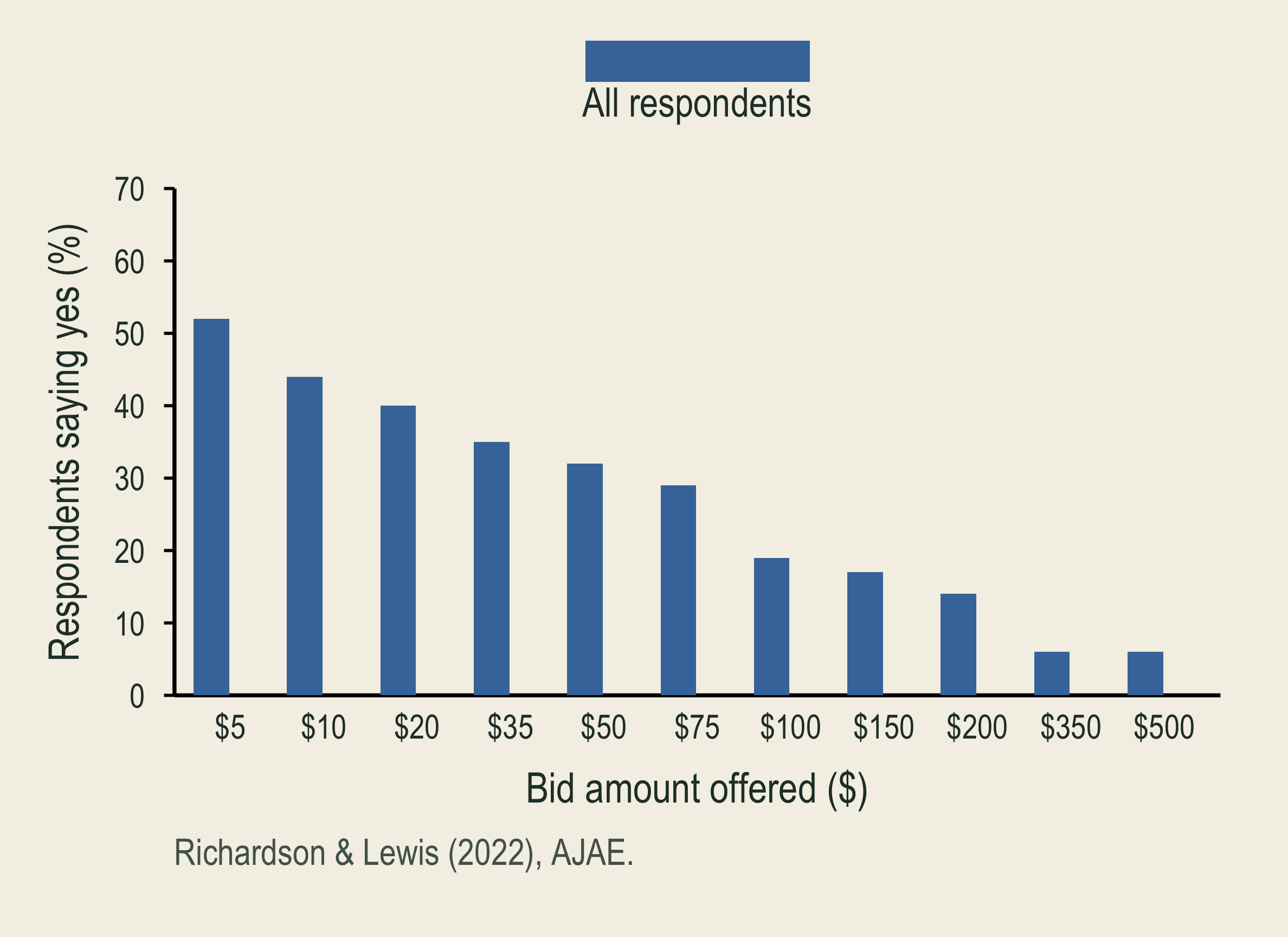
  • Survey question: would you give $X/year for five years? One of 11 amounts ($5–$500) was offered to each viewer.
  • Money-back rule: below the $100,000 target, the program would not proceed and donations would be refunded.

📉 Brown-Bear Responses and WTP

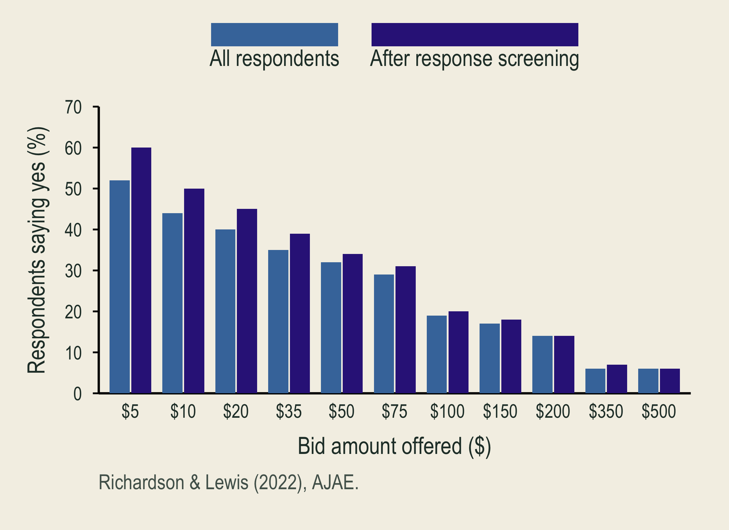
Among bear-cam viewers, acceptance of the annual donation generally falls as the proposed amount rises.

The response-screened sample is added. Both samples show lower acceptance at higher donation amounts.

  • Screening: remove protests, misunderstandings, and beliefs that answers cannot affect protection.
  • 14% excluded: 3,736 of 4,361 valuation respondents remain. Genuine zero WTP is retained.
  • Screened-sample mean WTP: $70–$140/year.

Implication: wildlife protection can benefit people watching from afar. These values can inform wildlife policy and damage assessments.

🧩 A Random Utility Model for Our Experiment

\[\begin{aligned} \text{Utility}_{ij}&=\alpha_j+\beta_c\,\text{Cash kept}_{ij}\\ &\quad+\color{#4477AA}{\beta_g\,\text{Conservation gift}_{ij}}+\varepsilon_{ij} \end{aligned}\]

\(i\): respondent; \(j\): option; \(\alpha_j\): baseline preference for an option.

  • Error term \(\varepsilon_{ij}\): reasons for your choice that we do not measure, such as how much you trust an organization.
  • Choose the highest total utility. We estimate the model from choices.
Actual dollars Cash kept Gift
Ducks Unlimited $7.50 $1
Trout Unlimited $7 $1
Keep all cash $8 $0

Recall p7: add $1 to the same recipient’s gift; give up \(x\) dollars of cash.

\[\begin{aligned} \Delta U&=\beta_g-\beta_c x=0\\ \text{MWTP}=x&=\frac{\beta_g}{\beta_c} \end{aligned}\]

  • Cash forgone per extra $1 delivered, holding other influences fixed.

💧 A Water-Quality Choice Experiment

Option B: larger nutrient and clarity improvements; NZ$6/month.

Option C: more rivers suitable for recreation; NZ$3/month.

Change from baseline A: no change B C
Rivers meeting nutrient limits (pp) 0 +5 +1
Water clarity (m) 0 +1 +0.5
Rivers suitable for recreation (pp) 0 +6 +8
Household cost (NZ$/month) 0 6 3
  • pp = percentage points. Which plan would you choose?
  • Estimated WTP: NZ$12.10/household/year for 10 cm more clarity.

🏛️ Valuing the National Park Service

Method: households chose among park/program cuts and ten years of extra federal taxes; researchers estimated WTP and scaled it nationally.
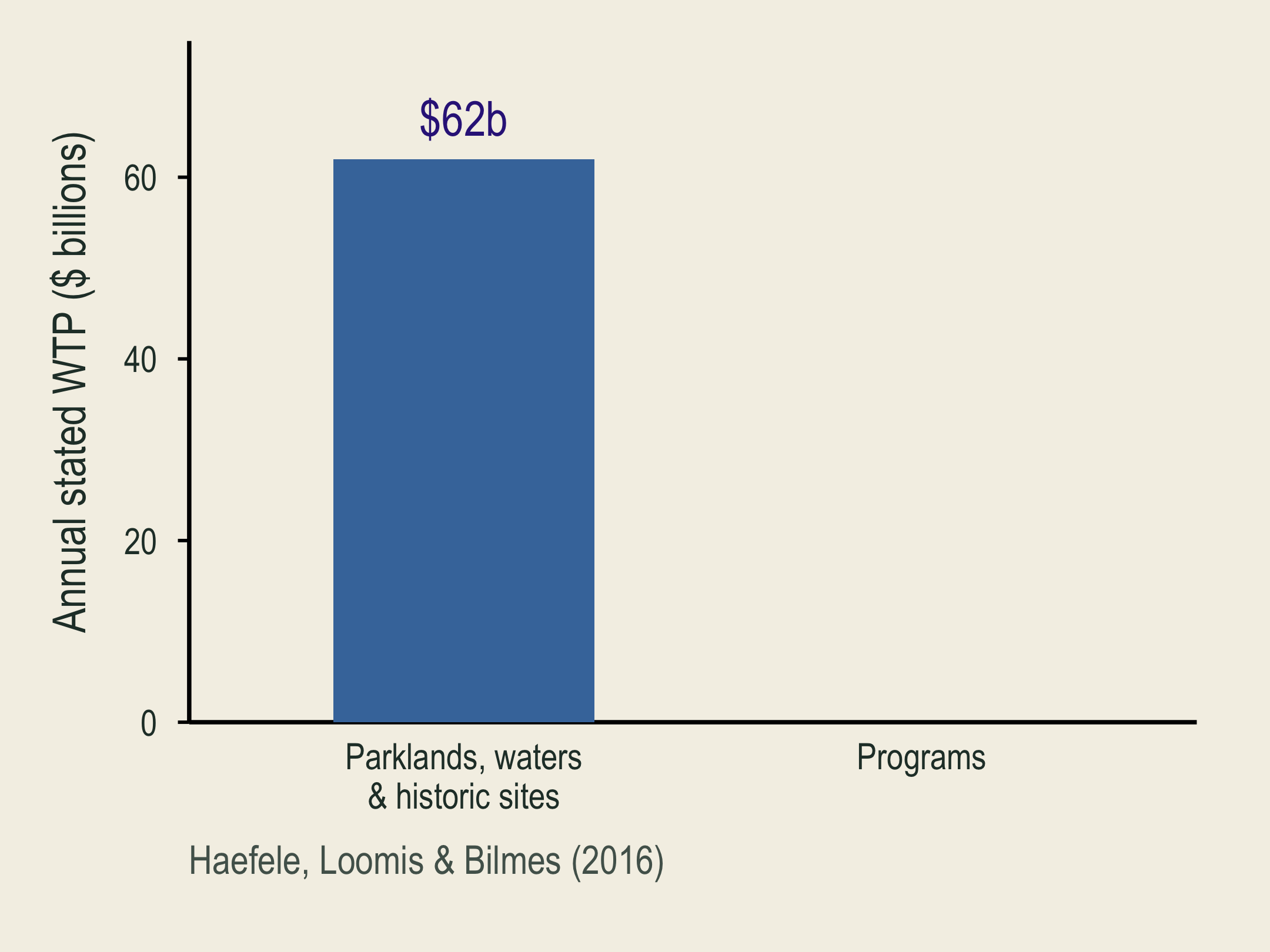
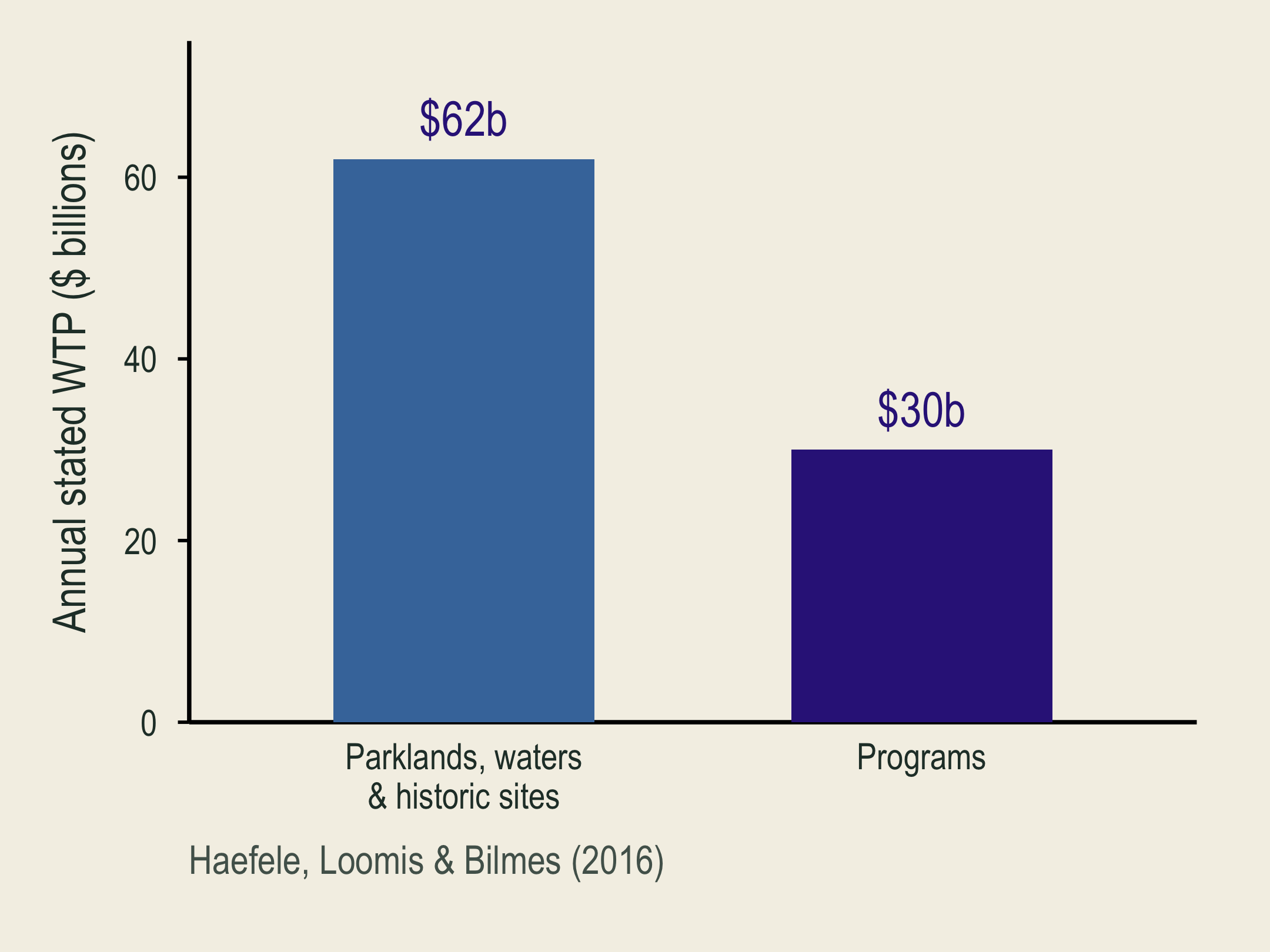
The parklands, waters, and historic sites component is revealed first: estimated annual stated WTP is 62 billion dollars.

Annual stated willingness to pay totals 92 billion dollars: 62 billion for National Park Service lands, waters, and historic sites, and 30 billion for programs.

  • Parks: $62 billion/year. Lands, waters, and historic sites.
  • Programs: $30 billion/year. Education, local preservation, and community recreation.

Total: $92 billion/year in estimated WTP, including use and nonuse values.

Quick check: which benefits would park entrance fees miss?

🏞️ Travel Cost and Recreation Demand

🏞️ A Free Recreation Site Still Has a Price of Access

Travel-cost step What the analyst uses
Observe behavior Trips, transport expense, travel time, and visitor characteristics
Estimate demand How visits change as generalized trip cost changes
Measure benefit Consumer surplus under the estimated recreation-demand curve

Travel spending helps identify demand. Spending itself is not the full recreation value.

📈 Travel Cost and Annual Visits

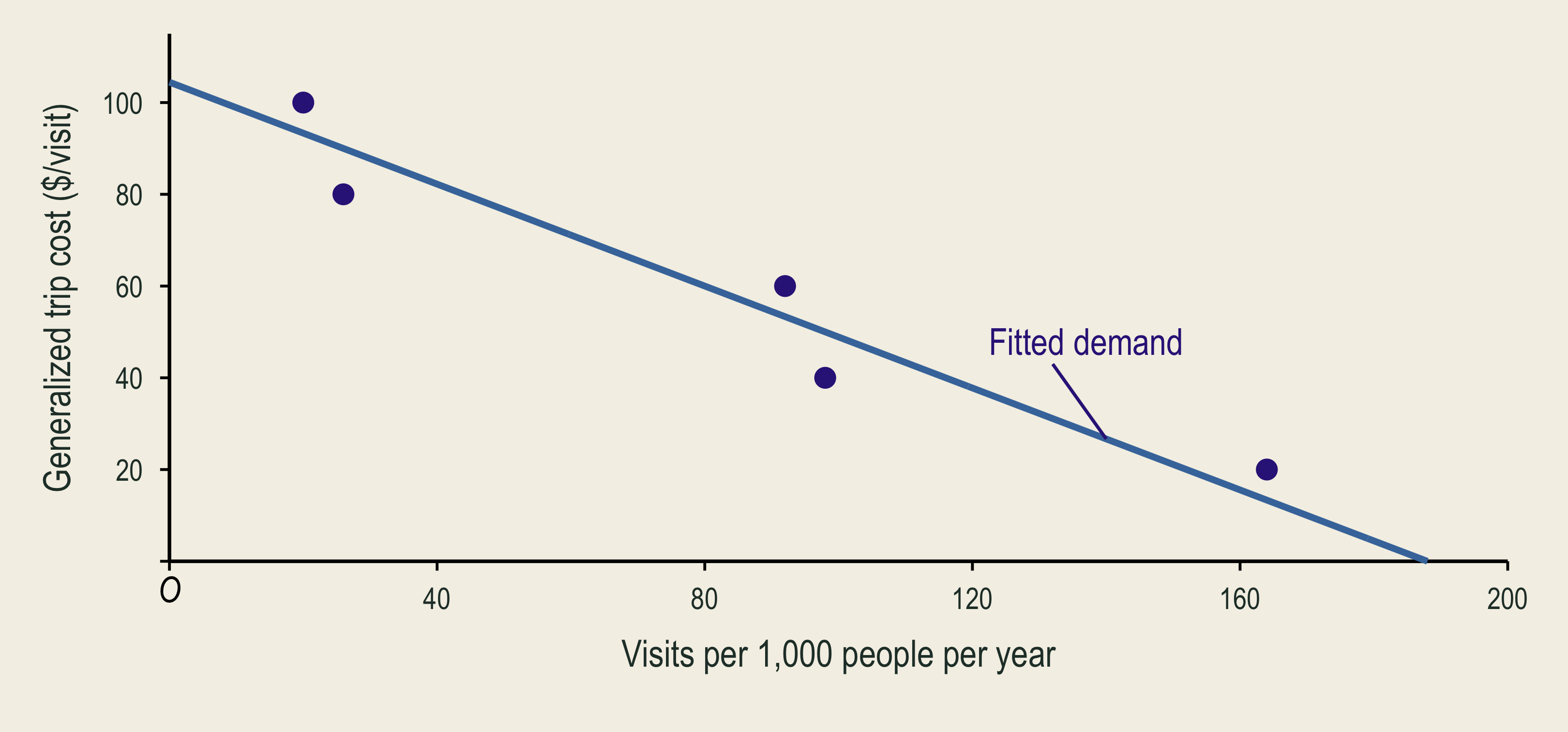
Five equal-sized regions. Trips per 1,000 residents/year.
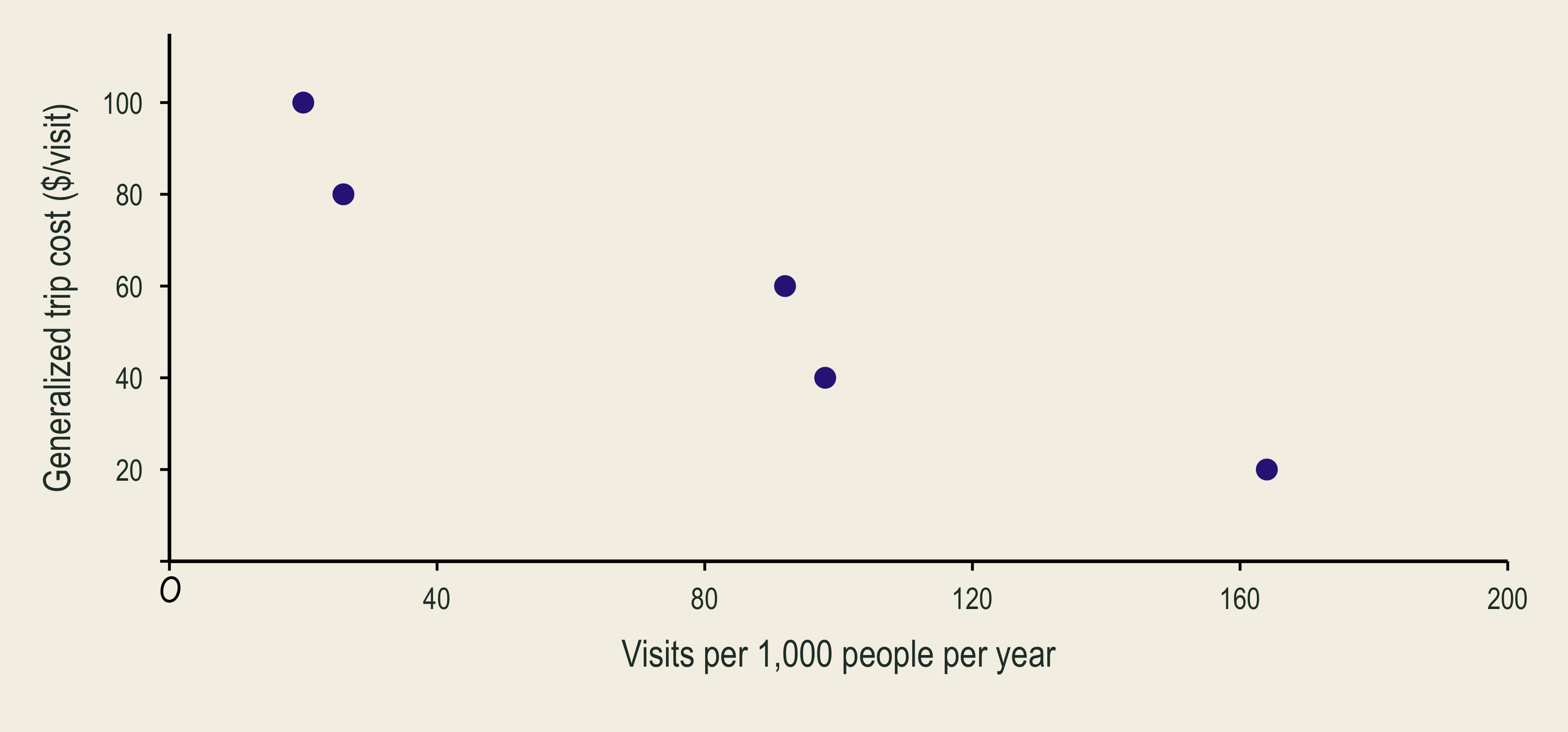
Five observations show fewer annual trips per one thousand residents at higher generalized trip costs.

Five scattered observations lie on either side of fitted recreation demand, Q-hat equals 188 minus 1.8 times generalized trip cost P.

\[\underbrace{\widehat Q}_{\text{predicted annual visits}}=188-1.8P\]

🔺 Visits and Consumer Surplus

\[\underset{\text{money + time cost per visit}}{P=\$60}:\qquad \widehat Q=188-1.8(60)=80\]
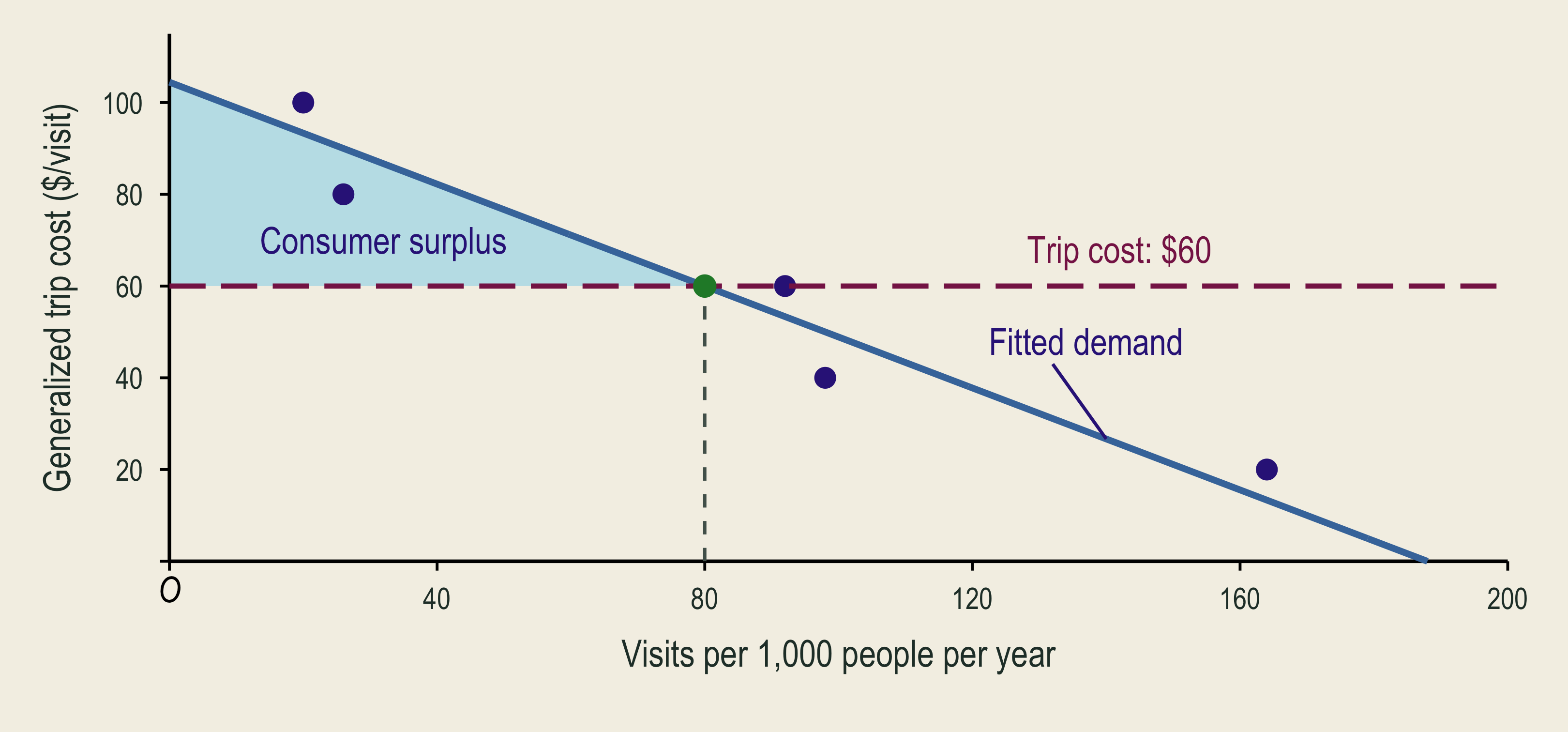
At a sixty-dollar generalized trip cost, predicted annual trips are eighty per one thousand residents. The shaded triangle above cost and below fitted inverse demand is consumer surplus.

\[CS\approx\$1{,}778\text{ per 1,000 people/year}\]

🌊 Recreation Loss From Lower Quality
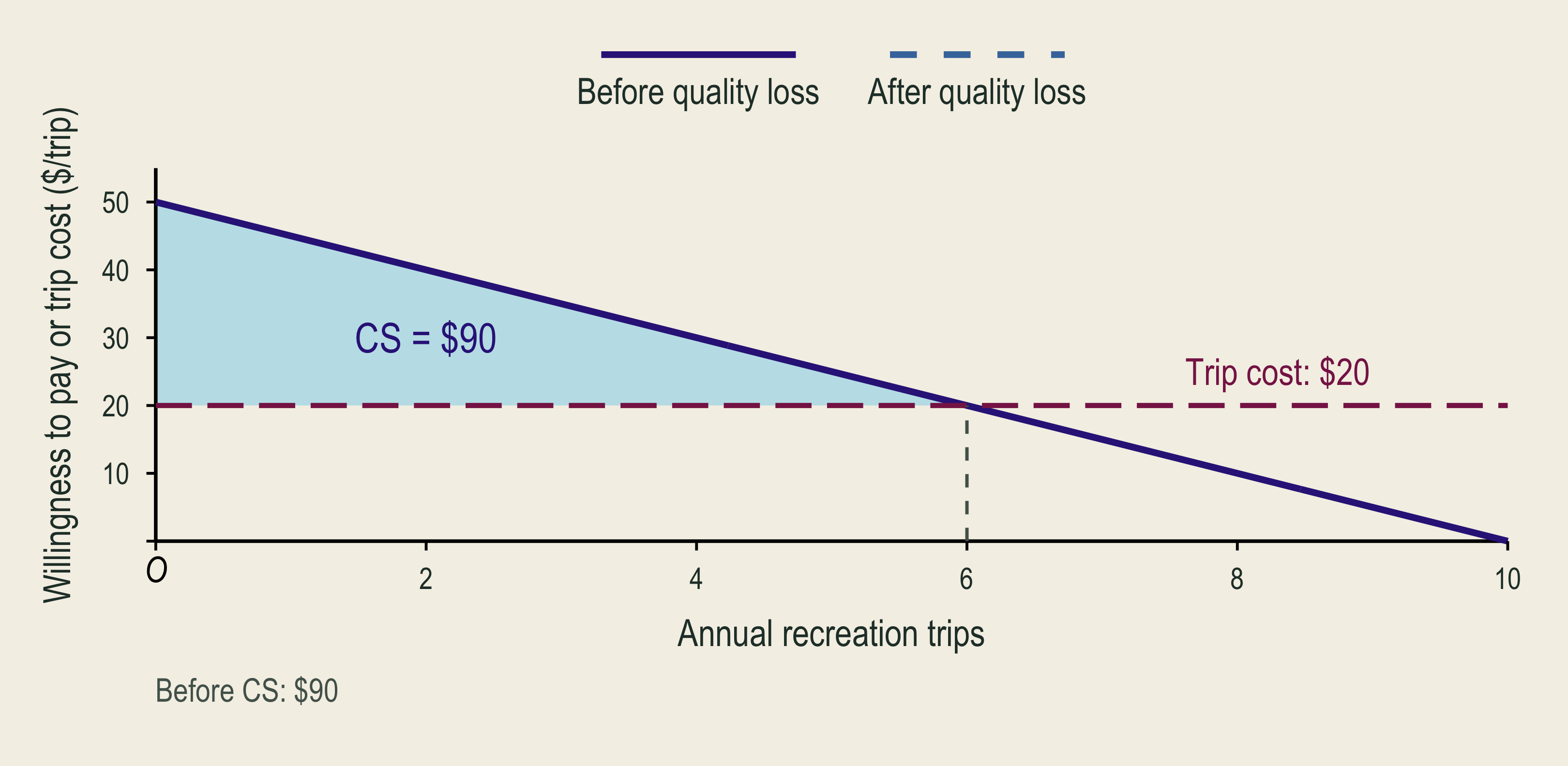
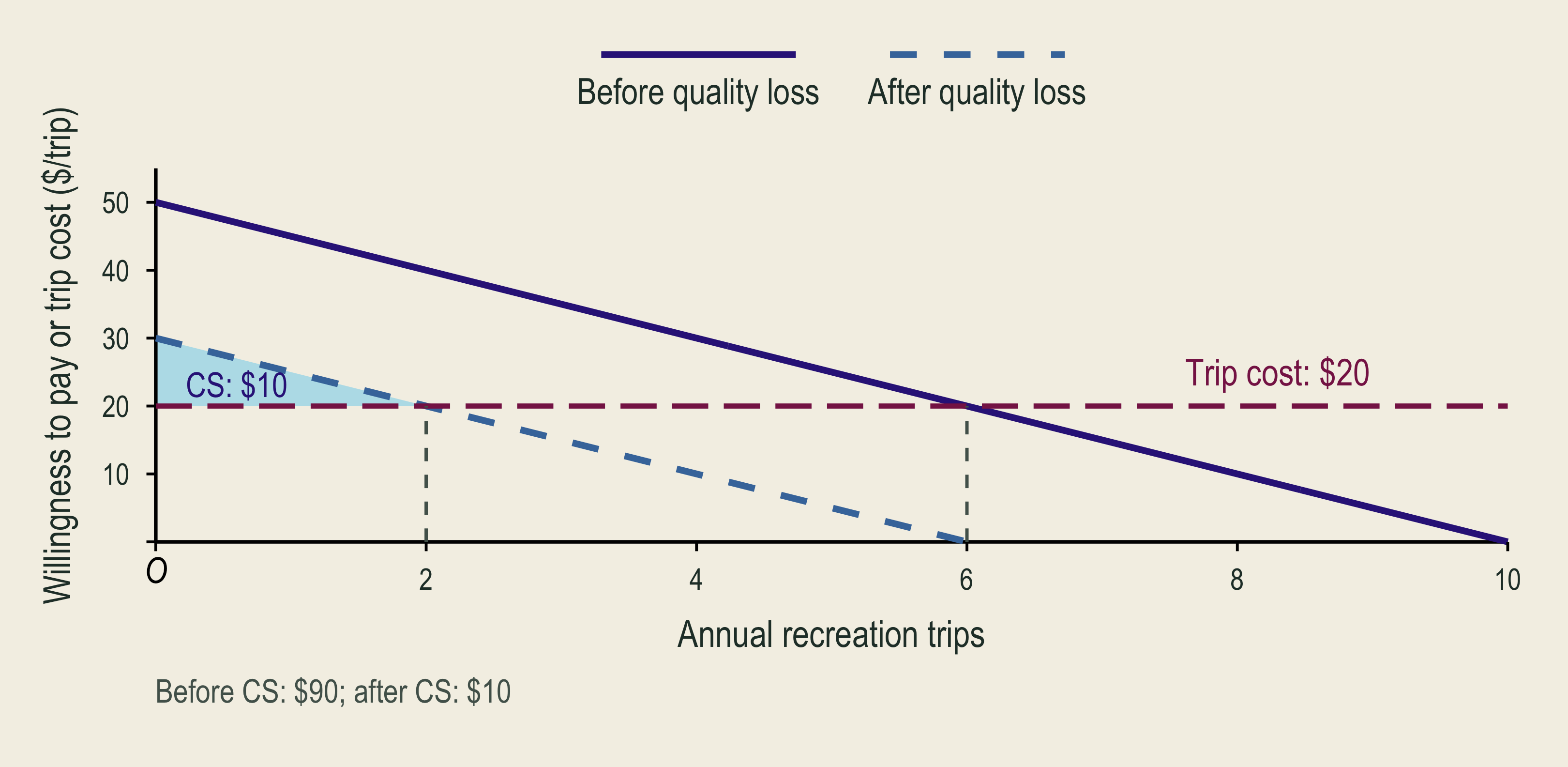
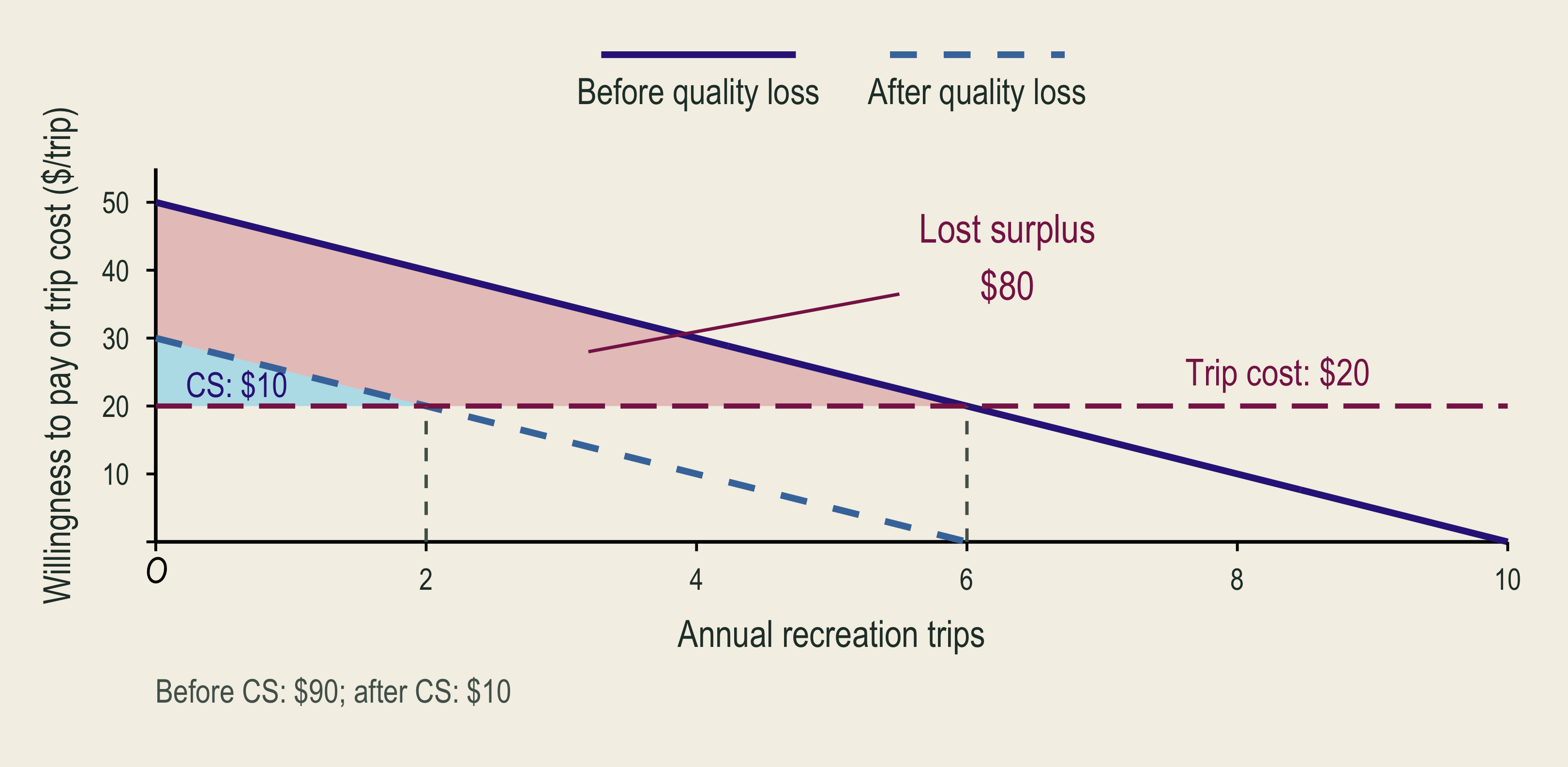
Before a quality loss, six annual visits at a twenty-dollar trip cost yield ninety dollars of consumer surplus.

After quality deteriorates, recreation demand shifts inward and consumer surplus falls.

The lost consumer-surplus area measures the recreation welfare loss from lower environmental quality in the classroom example.

  • Compare welfare before and after, allowing behavior to change.

🗺️ Site Choice and Substitution

1. Choose beach A

Preferred given its trip cost and quality.

2. Beach A closes

The preferred site becomes unavailable.

3. Choose again

Beach B, fewer trips, or stay home.

Welfare loss depends on how good and how costly the alternatives are. Close substitutes can soften the loss.

⚠️ Travel-Cost Estimates Depend on Modeling Choices

Question Why it matters
Was the trip for several purposes? If you stop at a park on the way to visit family, count the extra time and expense of the park detour.
How is travel time valued in dollars? 2 hours × assumed $15/hour = $30 in time cost.
Which substitute sites were available? A nearby alternative can reduce the loss from a closure.
Who never visited? Trip behavior cannot reveal their existence or bequest values.

🏖️ Minorca Beach Closures and Site Substitution

  • 573 visitors surveyed at 51 beaches in 2008.
  • Recorded beach choices, beach attributes, and trip costs.
  • Used a RUM to estimate recreation losses from oil-spill closures.
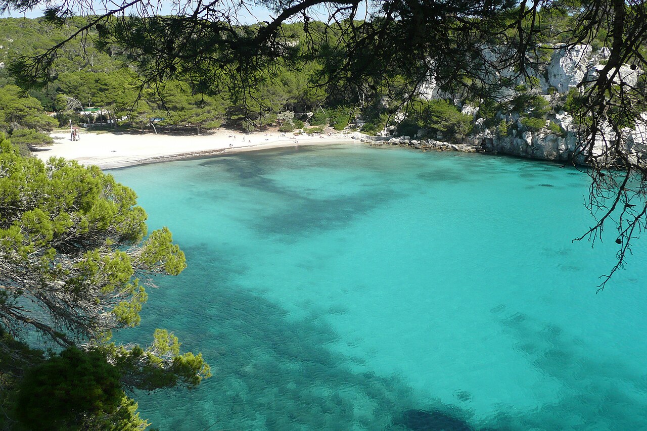
Cala Macarella in Minorca, with a sandy beach, pine-covered cliffs, and turquoise water.
Cala Macarella, Minorca, Spain
Closed beaches €/visit €/day
West beaches €0.24 €6,000
West and north beaches €1.73 €43,250

Implication: wider closures leave fewer alternative beaches, increasing visitors’ recreation losses. These estimates can inform oil-spill damage assessments.

🏠 Hedonic Pricing

🏠 Environmental Quality Is Part of a Housing Bundle
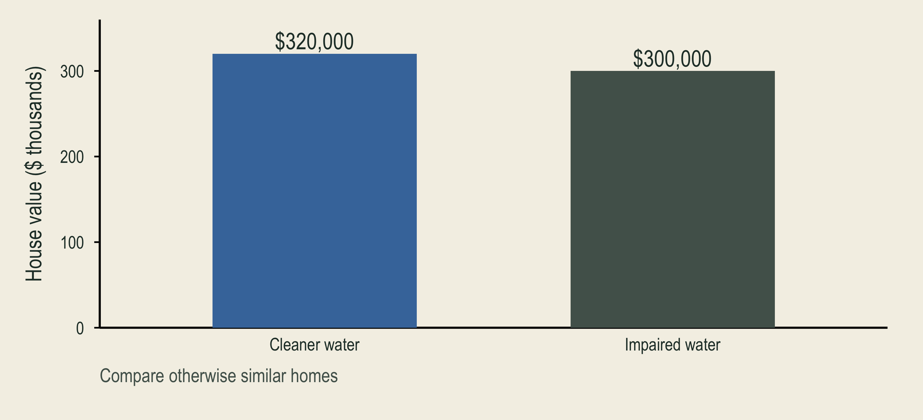
Otherwise similar homes near cleaner water have a higher illustrative price. The environmental contribution must be separated from the rest of the housing bundle.

  • A hedonic property model separates an environmental attribute from the rest of the housing bundle.

🔎 What Makes a Hedonic Comparison Credible?

\[\begin{aligned} \text{HomePrice}_i&=\alpha+\color{#4477AA}{\beta\,\text{Environmental quality}_i}\\ &\quad+\gamma\,\text{Home features}_i+\delta\,\text{Location}_i+\varepsilon_i \end{aligned}\]

Error term: \(\varepsilon_i\) captures unmeasured influences on home \(i\)’s price.

Other price determinant Evidence to seek
Different homes Size, age, lot, and repeat sales
Different locations Schools, commuting, and nearby amenities
Other changes over time A credible comparison group and timing
  • \(\beta\) measures the association between environmental quality and home price, holding other measured factors fixed.

🦺 Jobs Also Bundle Pay, Conditions, and Risk

\[\begin{aligned} \text{Wage}_i&=\alpha+\color{#D55E00}{\beta\,\text{Fatality risk}_i}\\ &\quad+\gamma\,\text{Worker traits}_i+\delta\,\text{Job features}_i+\varepsilon_i \end{aligned}\]

Error term: \(\varepsilon_i\) captures unmeasured influences on worker \(i\)’s wage.

Job characteristic Safer job Riskier job
Known workplace risk Lower Higher
Compensating pay Lower Higher
  • A hedonic wage model estimates the pay–risk trade-off, holding other job and worker characteristics constant.
  • \(\beta\) measures the additional pay associated with a higher fatality risk, holding other measured factors fixed.

📚 Benefit Transfer

📚 Benefit Transfer and Uncertainty

  • Benefit transfer: use existing estimates for a new policy.
  • Meta-analysis: study why published estimates differ.
    • Combine studies to compare sites, populations, and methods.
  • Match the change, population, units, and time period.
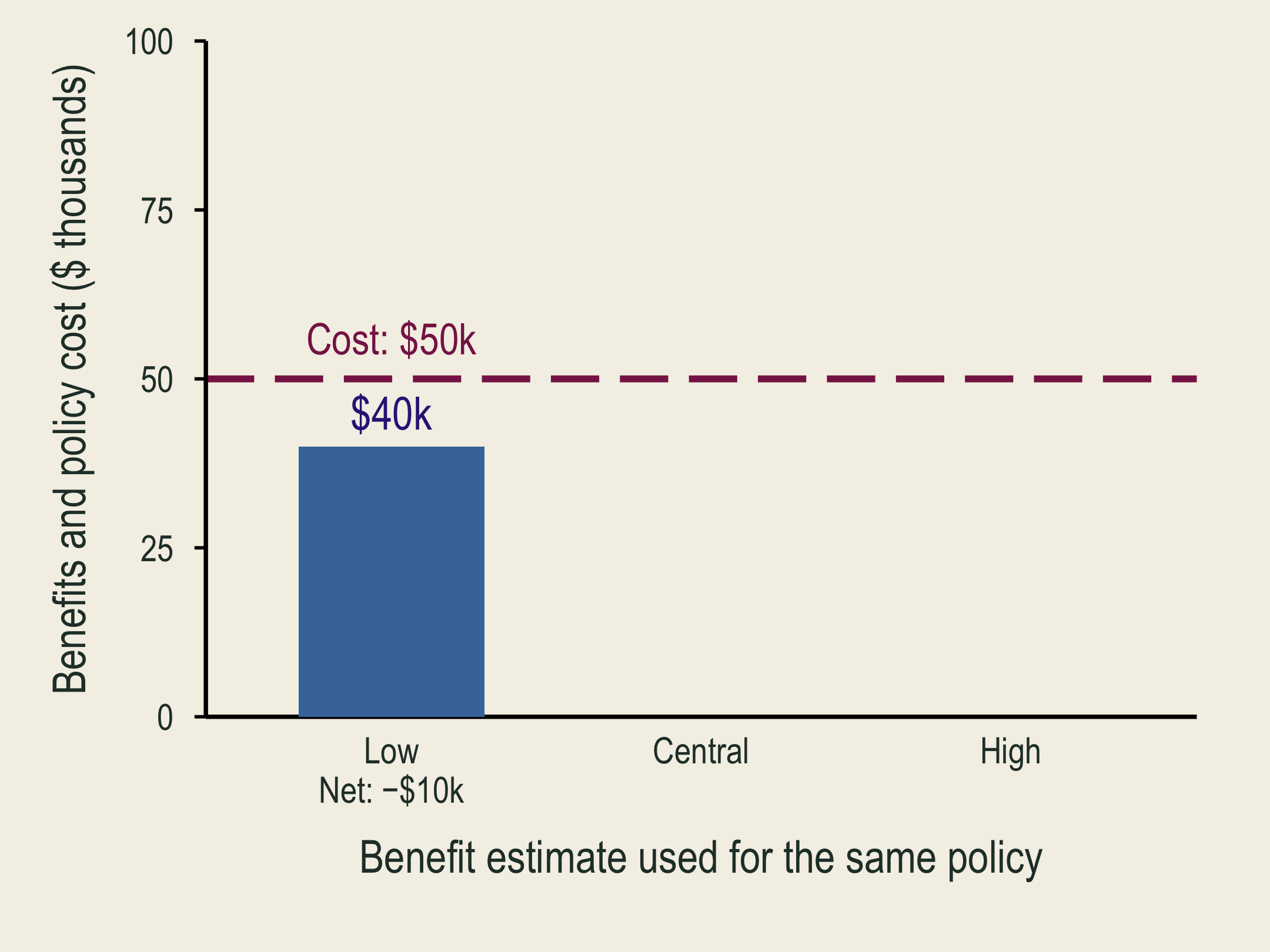
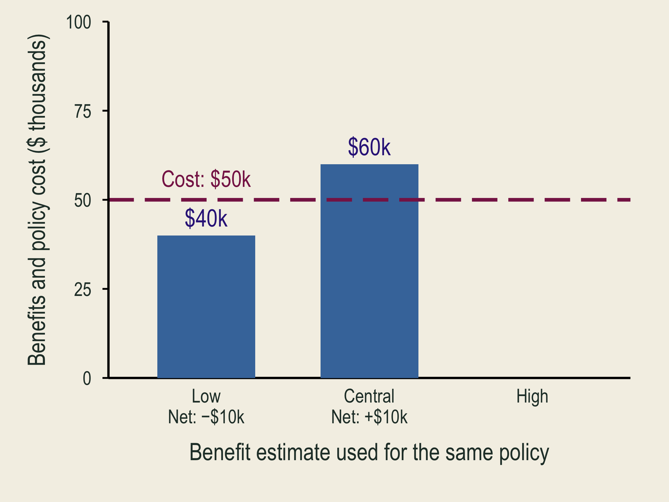
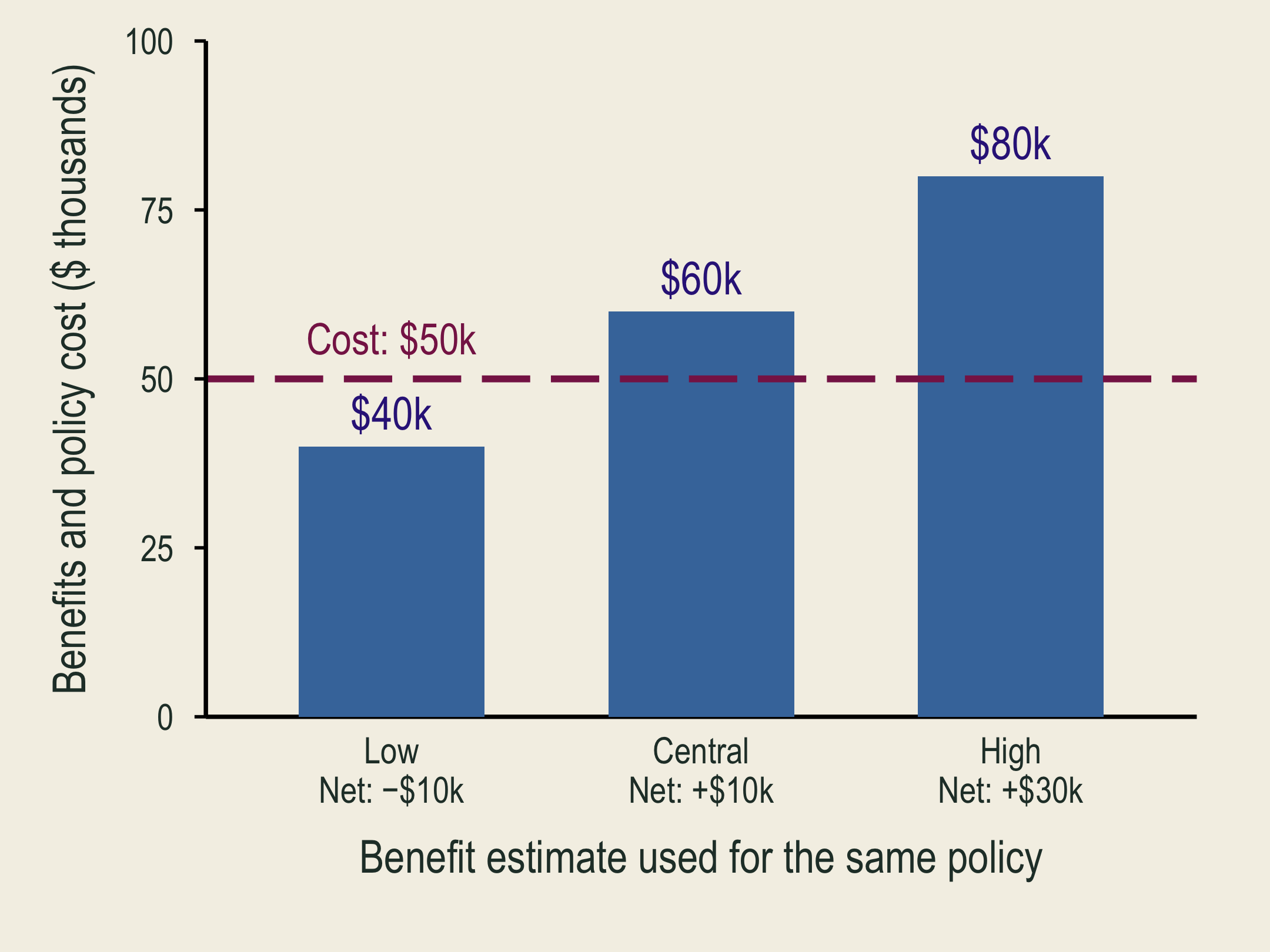
A low benefit estimate is below the fixed policy cost, so net benefit is negative.

With the central benefit estimate, the same policy has positive net benefit.

Low, central, and high benefits imply different net benefits despite an unchanged policy cost.

Low, Central, and High are alternative benefit estimates for the same policy, not different groups. Cost stays at $50,000. Does the estimate change the decision?

❄️ The Value of Polar Bears
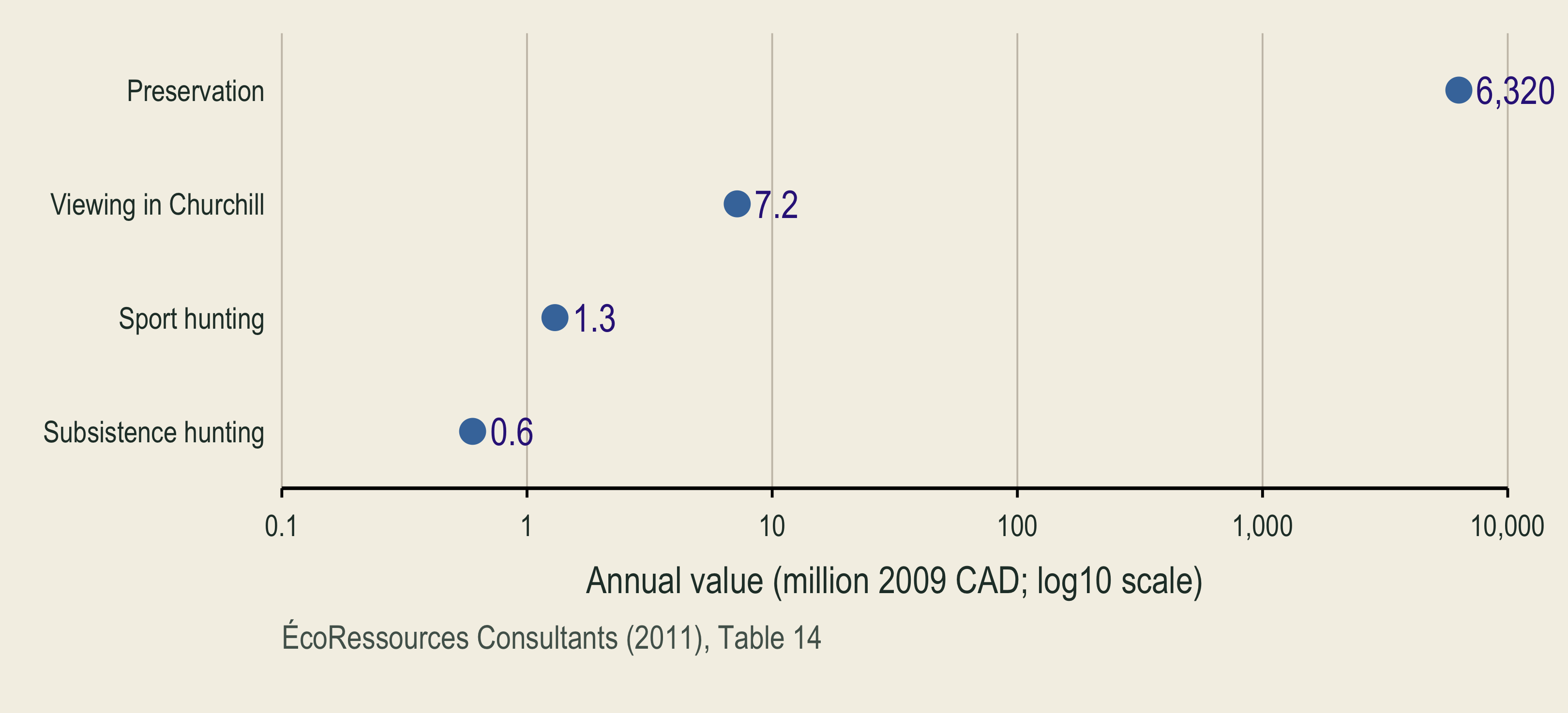
A value-category hierarchy separates human-centered and intrinsic values. Total economic value branches into active and passive use. Sport hunting, subsistence hunting, and viewing are annotated with 1.3, 0.6, and 7.2 million 2009 Canadian dollars per year. One 6,320 million preservation estimate spans indirect use, option, existence, and bequest values. Cultural and intrinsic values have no dollar estimate.

Different valuation methods capture different types of value (See Table 1 in below reference).

🩺 Valuing Mortality-Risk Reductions

🩺 Value of Statistical Life (VSL)

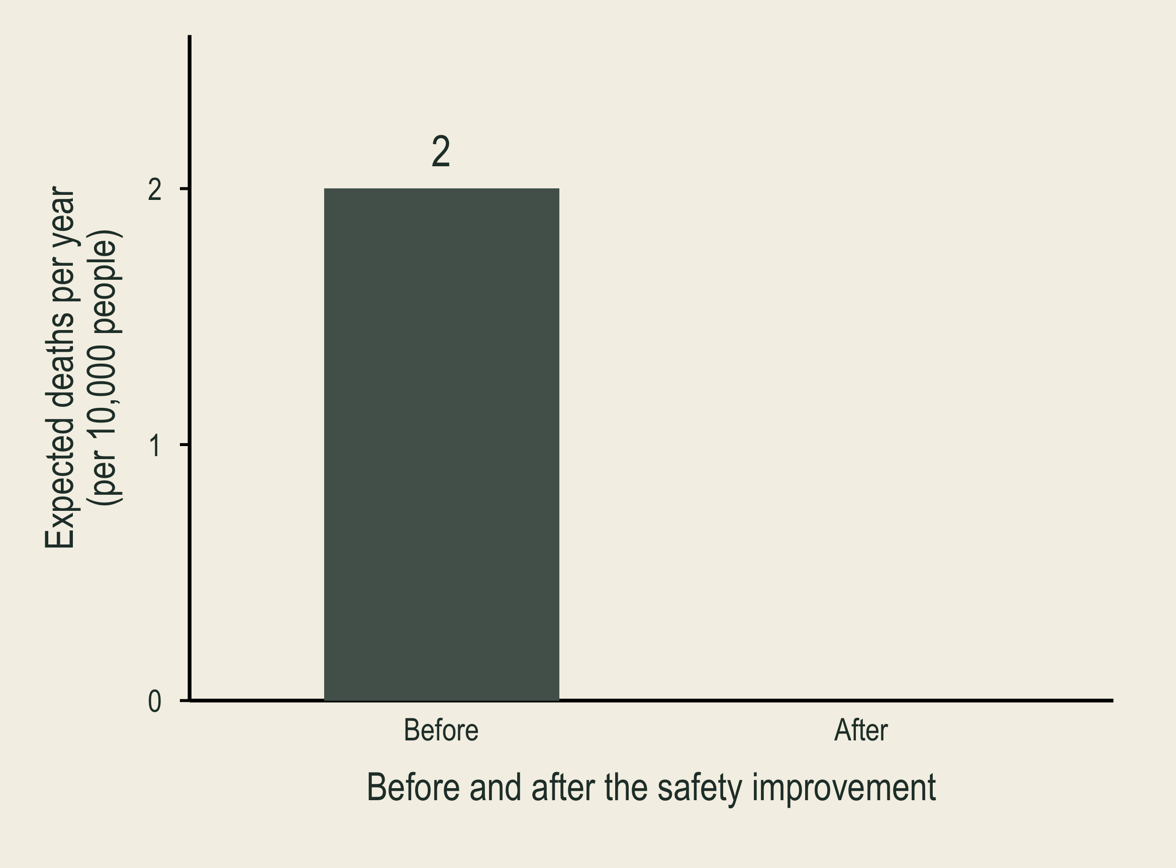
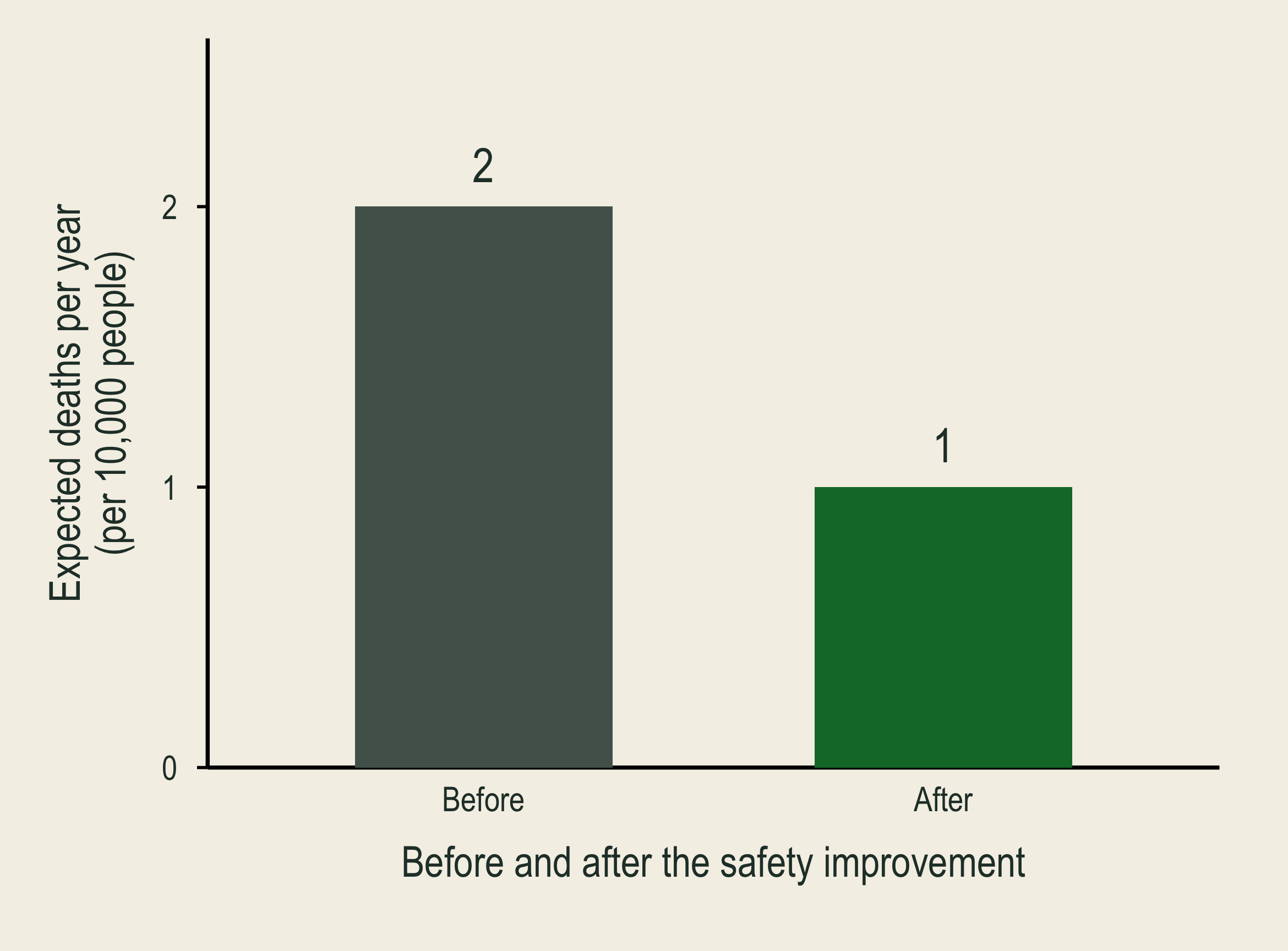
At annual mortality risk two in ten thousand, ten thousand people face two expected deaths per year.

Reducing each person's annual risk to one in ten thousand lowers expected deaths from two to one among ten thousand people.

VSL values reductions in mortality risk, not an identified person’s life.

Suppose each person would pay $1,000 to reduce their annual risk of death by 1 in 10,000.

\[VSL=\frac{\$1{,}000}{1/10{,}000}=\$10\text{ million}.\]

  • In 2025 dollars, DOT uses $14.2 million and HHS uses $14.1 million.
  • EPA uses a central VSL of $10.7 million (2022 dollars).
  • Clean Air Act: mortality-risk benefits ≈90% of projected 2020 monetized benefits (EPA, 2011); share varies by policy.

🚗 Speed vs. Safety: Travel Time and Fatal Crash Risk

Byeong-Hak Choe and Stephen Newbold
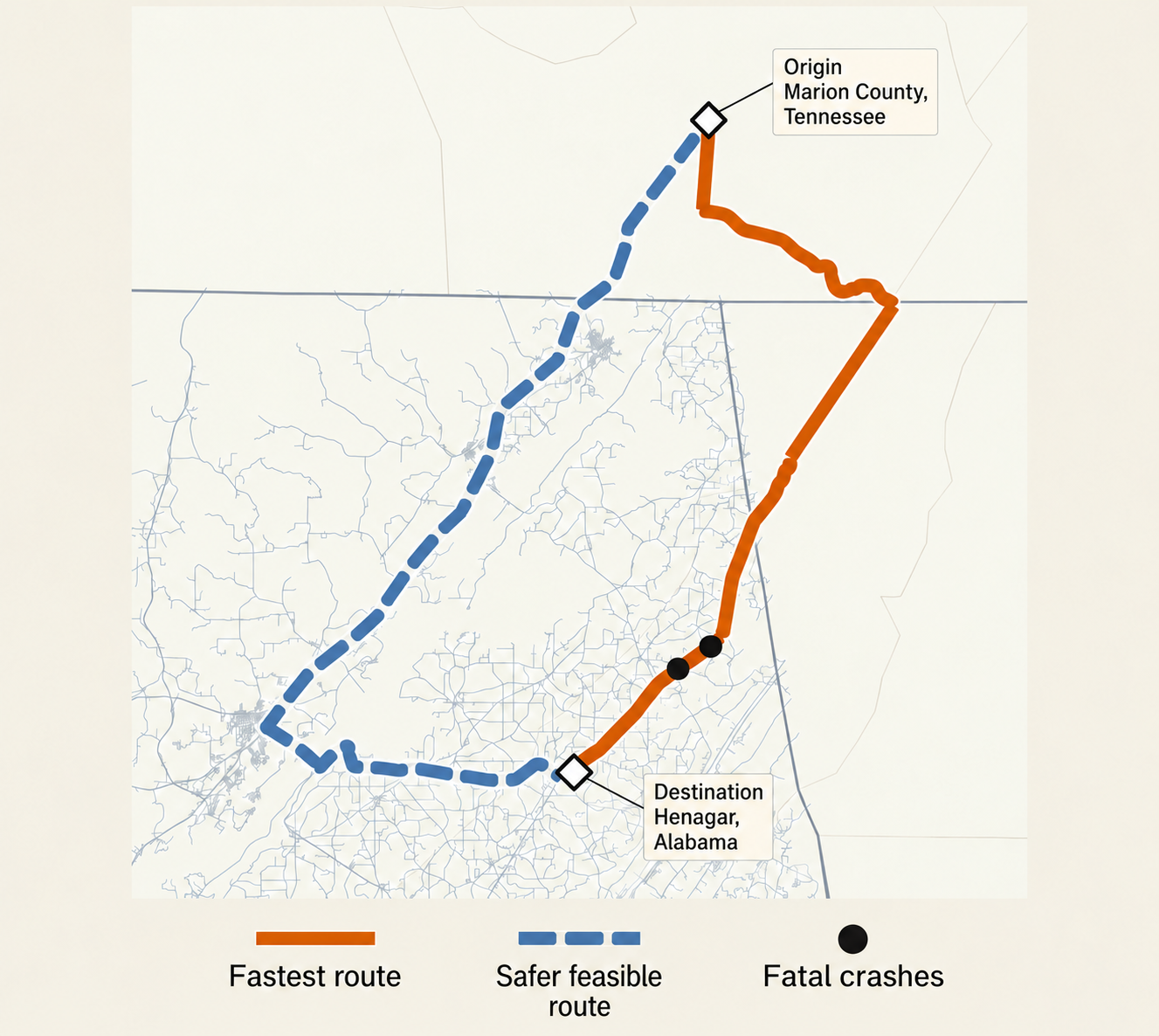
Routes from Marion County, Tennessee, to Henagar, Alabama, with repositioned origin and destination labels. A bottom legend identifies the solid orange fastest route, dashed blue safer feasible route, and black fatal-crash dots.

Marion County, Tennessee, to Henagar, Alabama.
  • Do faster journeys save enough time to justify added fatal-crash risk?
  • Time benefit: time saved × value of travel time.
  • Risk cost: added expected fatalities × VSL.
  • We use VSL as an input, rather than estimate it here.