Classwork 1
Market Diagnostic: Fish Harvest from a Finite Stock
Purpose
This is an ungraded diagnostic. Work independently first, compare with a partner, then revise in another color. The goal is to identify which microeconomics tools need review—not to produce a score.
Scenario
The weekly market for fish from a single fishery has:
Q_D=120-4P
Q_S=-40+4P
Quantities are measured in metric tons of fish per week, and price in hundreds of dollars per metric ton.
Task 1 · Equilibrium
- Solve for the competitive equilibrium price and quantity.
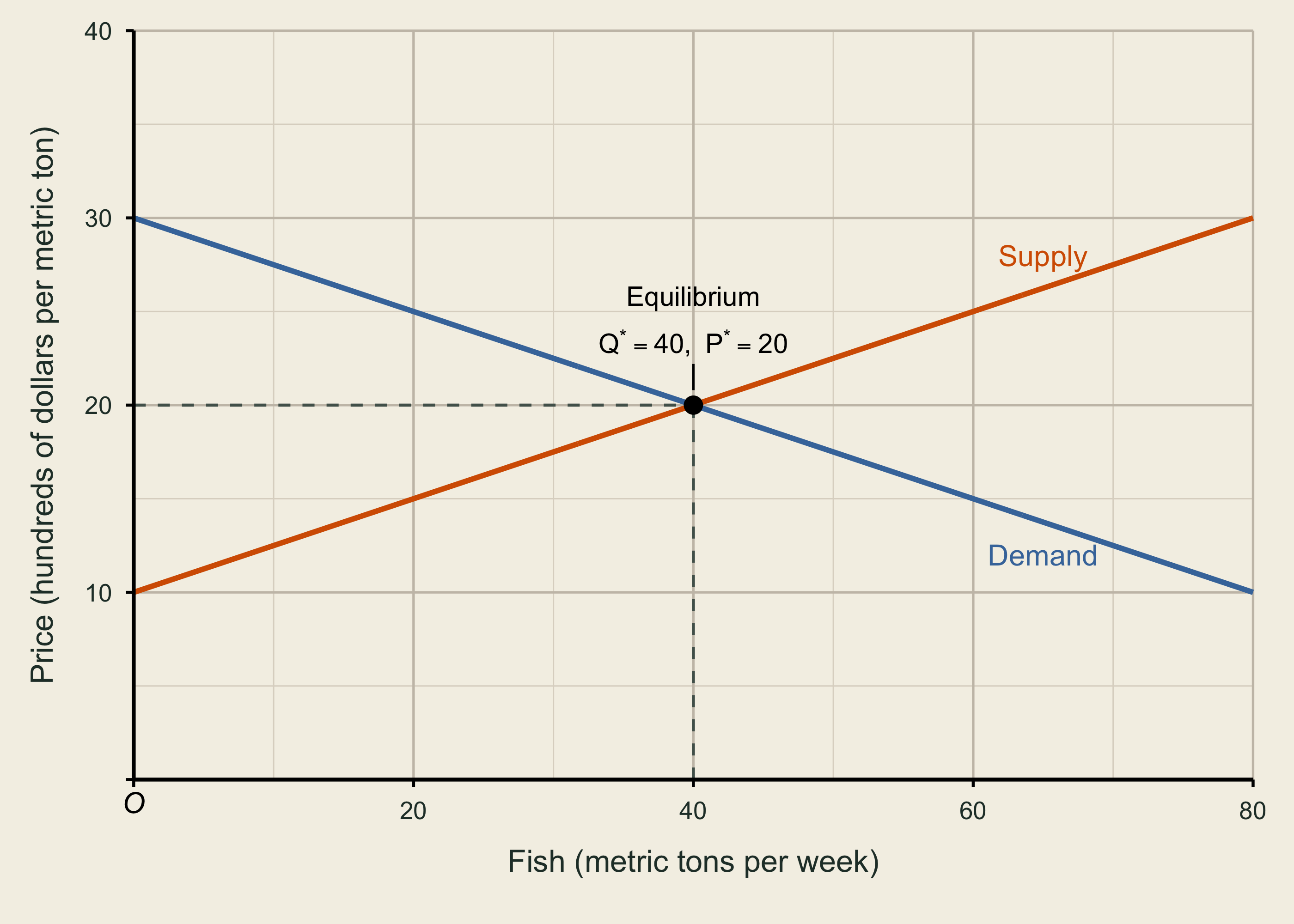
- Draw labeled demand and supply curves.
- Show the equilibrium on the graph.
TipCheck your result
Set 120-4P=-40+4P. The equilibrium is P^*=20 ($2,000 per metric ton) and Q^*=40 metric tons per week.
Task 2 · Surplus
- Find the demand choke price.
- Find the supply intercept price.
- Calculate consumer surplus and producer surplus.
- Using your graph, identify:
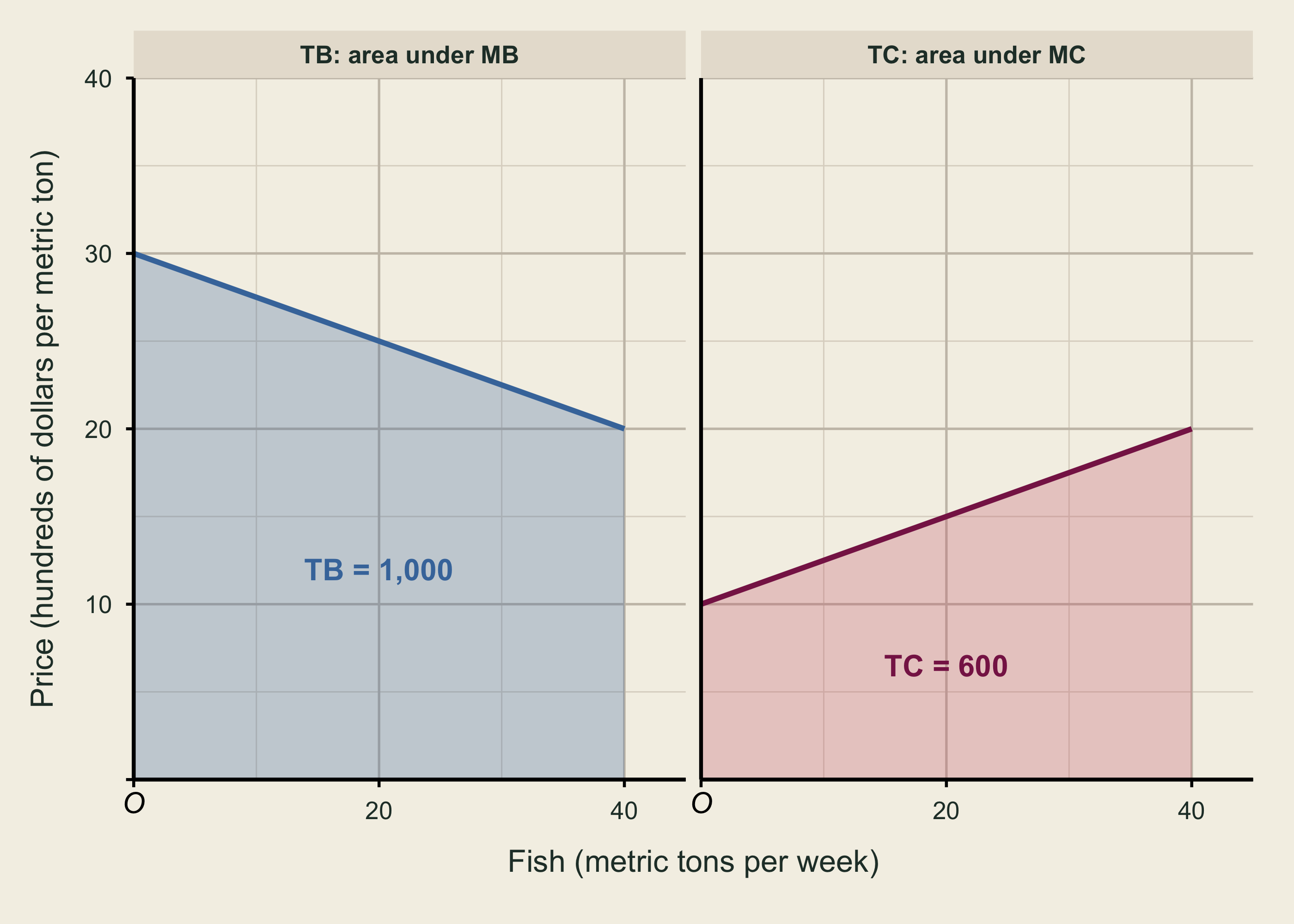
- total benefit (TB) as the area under MB from Q=0 to the equilibrium quantity; and
- total cost (TC) as the area under MC over the same quantities.
- Calculate TB and TC. Verify that TB-TC=CS+PS.
TipCheck your result
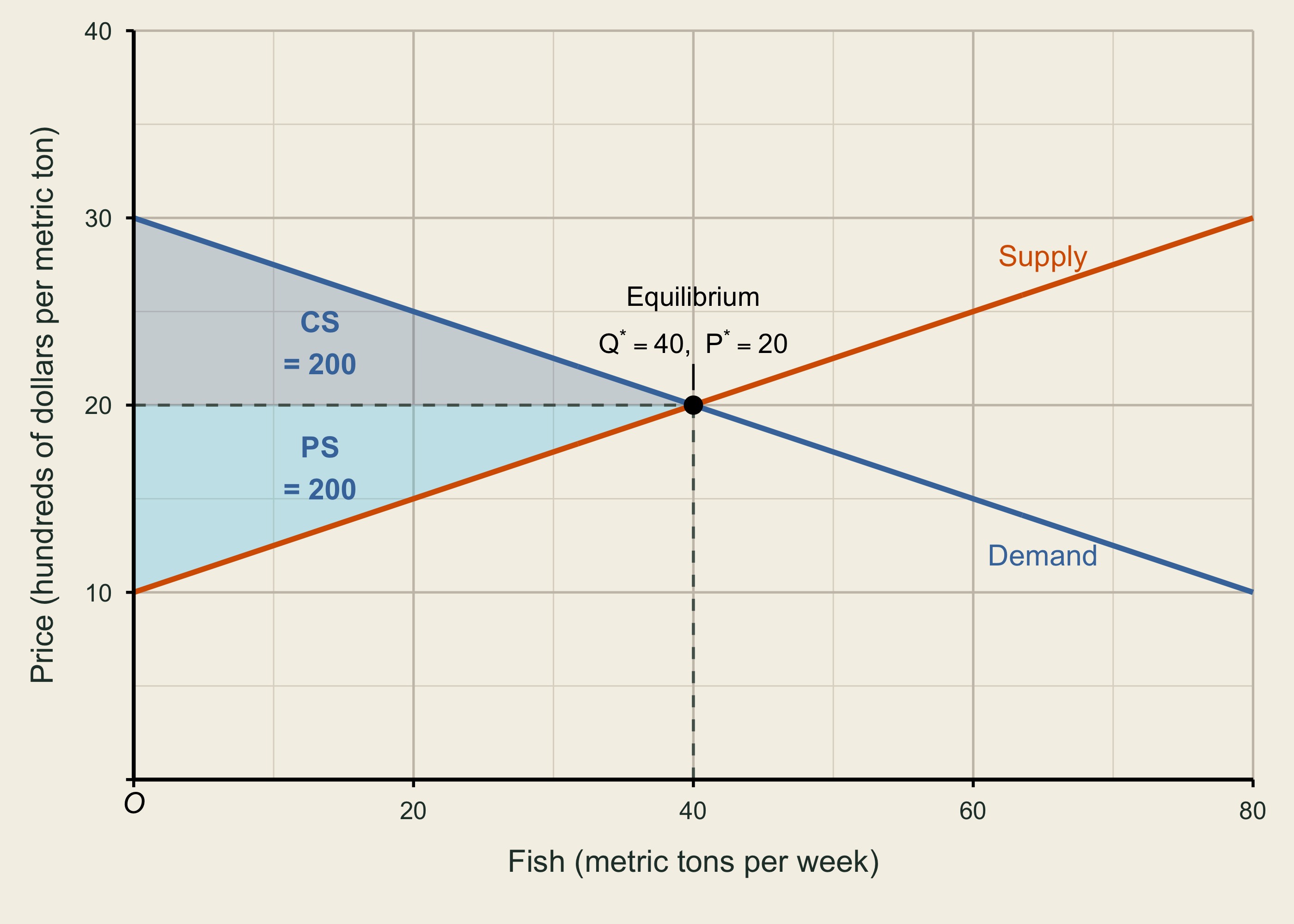
Inverse demand is P=30-0.25Q; inverse supply is P=10+0.25Q.
CS=\tfrac12(30-20)(40)=200
PS=\tfrac12(20-10)(40)=200
Each surplus is 200 in hundreds of dollars per week, or $20,000 per week.
Graphically, TB is the entire area under MB through Q^*=40, while TC is the entire area under MC over those same 40 metric tons:
TB=\tfrac12(30+20)(40)=1{,}000
TC=\tfrac12(10+20)(40)=600.
Therefore,
TB-TC=1{,}000-600=400=CS+PS.
These areas are measured in hundreds of dollars per week, so TB=\$100{,}000, TC=\$60{,}000, and total surplus is \$40{,}000 per week.
Task 3 · A harvest quota that limits quantity
Suppose the government limits total fish harvest to 30 metric tons per week. Assume the sellers who supply this restricted quantity receive the quota-created price difference.
- Does the quota actually limit harvest? Explain by comparing it with the competitive quantity.
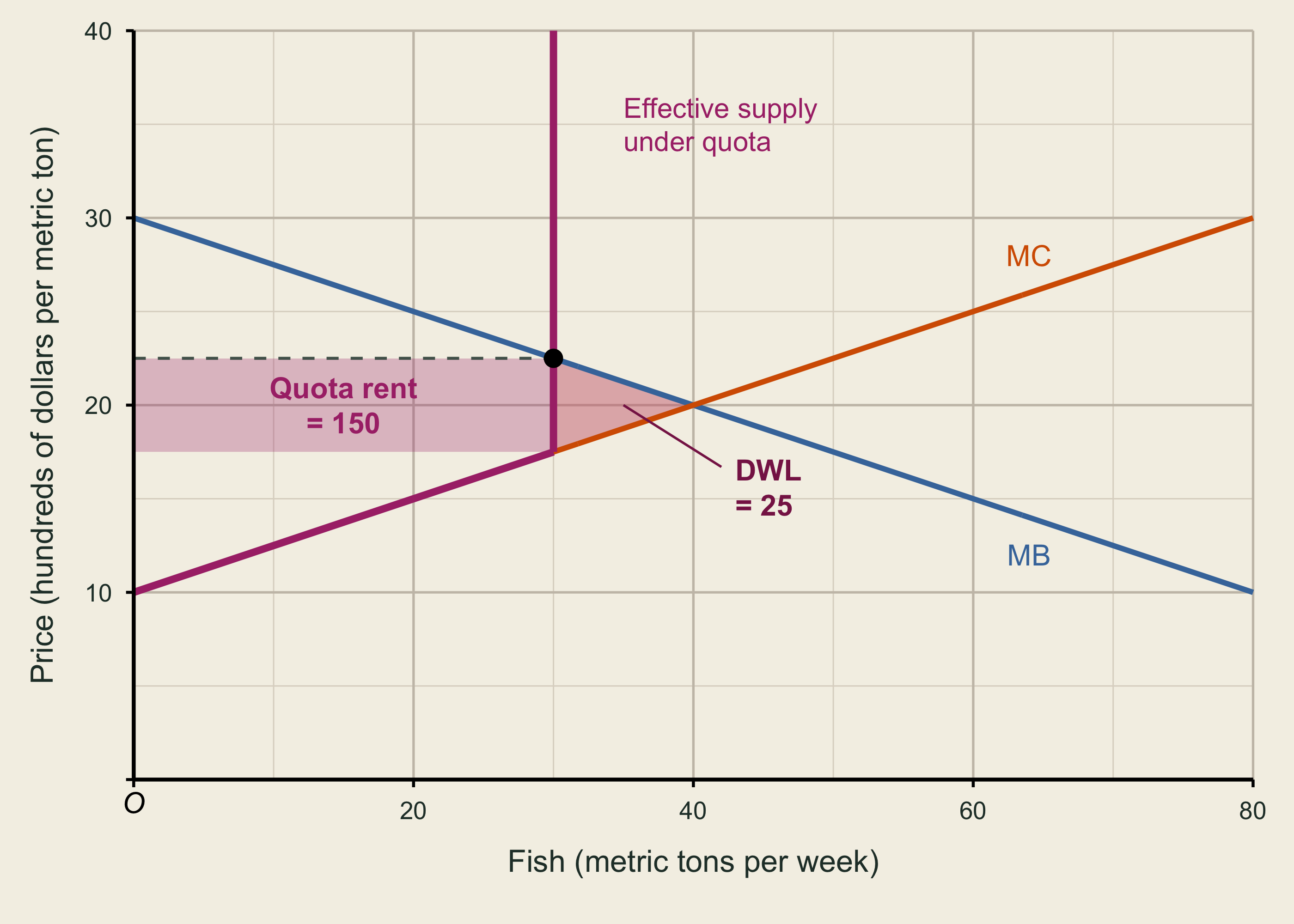
- On your graph, keep the original MC curve visible. Draw the effective market supply following MC through 30 metric tons and then becoming vertical at the quota.
- At Q=30, use demand to find the market price and use MC to find the marginal harvesting cost.
- Shade and calculate the quota rent and the deadweight loss.
- Calculate CS, PS including quota rent, and total surplus under the quota.
TipCheck your result
Yes. The quota limits harvest because 30 metric tons is below the competitive quantity of 40.
At Q=30,
P_D=30-0.25(30)=22.5,
while
MC=10+0.25(30)=17.5.
The quota keeps sellers from expanding output even though the market price exceeds the marginal cost of the 30th metric ton. The resulting quota rent is
(22.5-17.5)(30)=150,
or $15,000 per week.
The consumer-surplus triangle is 112.5. Producer surplus excluding quota rent is also 112.5, so producer surplus including quota rent is 262.5. Total surplus is therefore 375, all in hundreds of dollars per week.
The deadweight-loss triangle between Q=30 and Q=40 is 25 hundreds of dollars per week, or $2,500 per week.
Task 4 · Demand shock
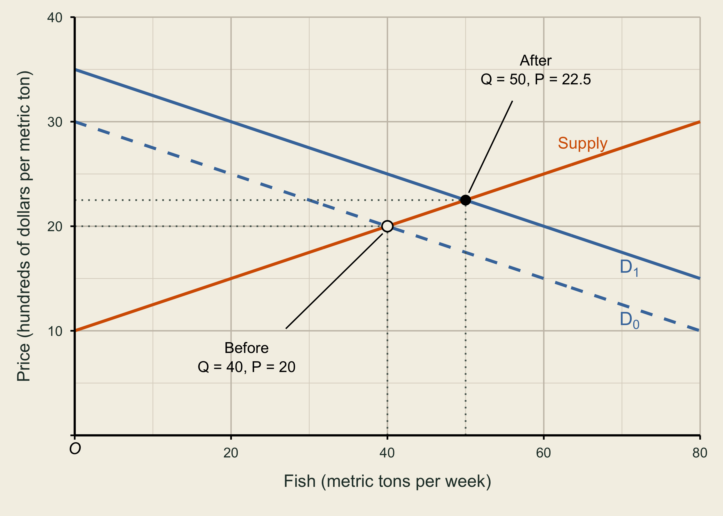
A surge in restaurant demand increases demand to:
Q_D'=140-4P
- Find the new equilibrium.
- Calculate the percentage change in equilibrium price and quantity. Which changes more in percentage terms?
TipCheck your result
The new equilibrium is P'=22.5 and Q'=50.
Using the original equilibrium, P^*=20 and Q^*=40, as the baseline:
\begin{aligned} \%\Delta P &=\frac{P'-P^*}{P^*}\times 100\\ &=\frac{22.5-20}{20}\times 100\\ &=12.5\%. \end{aligned}
\begin{aligned} \%\Delta Q &=\frac{Q'-Q^*}{Q^*}\times 100\\ &=\frac{50-40}{40}\times 100\\ &=25\%. \end{aligned}
Therefore, quantity rises more than price in percentage terms.
Task 5 · Add the stock
The fishery begins with 180 metric tons of harvestable fish biomass and no biological growth or recruitment during this short planning horizon.
- How many weeks can the original equilibrium harvest flow continue?
- Which information is missing if fishers choose harvest using only this week’s supply curve?
- Write one sentence distinguishing the stock from the flow.
TipCheck your result
For week t, use the stock accounting identity
S_{t+1}=S_t+G_t-H_t.
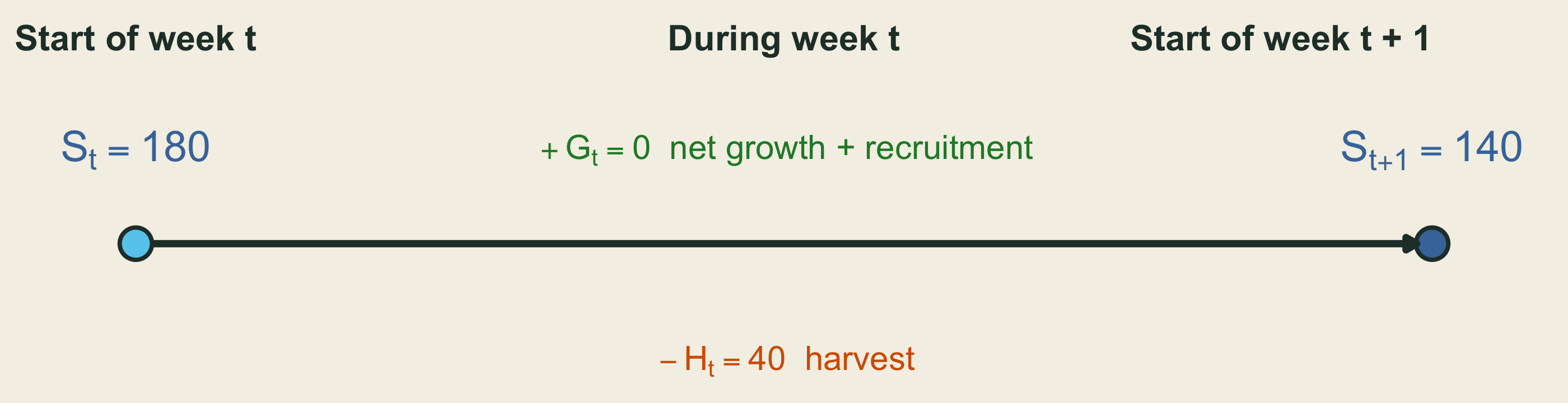
Because G_t=0 and harvest remains H_t=40 metric tons per week, the stock after n weeks is
S_n=S_0-nH=180-40n.
The stock is exhausted when S_n=0:
\begin{aligned} 0&=180-40n,\\ 40n&=180,\\ n&=\frac{180}{40}=4.5\text{ weeks}. \end{aligned}
Thus, the stock supports four complete weeks of 40 metric tons each, leaving 20 metric tons for one-half of the fifth week.
This exercise sets biological growth and recruitment to zero. The weekly supply curve omits the value of leaving fish available for future use and how today’s harvest affects future opportunities.
The stock is the fish biomass available in the water at a point in time; the flow is the fish harvested per week.
Exit sentence
Complete:
The ordinary market graph helps me see ________, but a natural-resource model must also track ________.
TipSample answer
The ordinary market graph helps me see prices, quantities, and gains from trade today, but a natural-resource model must also track how today’s harvest changes the resource stock and future opportunities.