Homework 1
Externalities, Resource Access, and Public Goods
Instructions
Due: Wednesday, September 23, 2026, at 9:30 A.M. Eastern Time.
Bring a written paper copy and submit it at the beginning of class.
Show your equations, algebra, and units. Label graph axes, curves, prices, and quantities; a neat hand-drawn graph is sufficient. Use areas of triangles, rectangles, and trapezoids to calculate welfare; calculus is not required. For short essays, explain the economic mechanism and support your reasoning with the case details. Suggested lengths apply to each response, not to the entire question set.
We use the lecture notation: MB for marginal benefit, PMC for private marginal cost, EMC for external marginal cost, and SMC=PMC+EMC for social marginal cost. For positive externalities, EMB is external marginal benefit and SMB is social marginal benefit. Prices and marginal values are in dollars per unit; total surplus, damage, revenue, and spending are in dollars for the stated period.
Do not use generative AI for any part of this homework, including reading or summarizing sources, solving calculations, drafting or revising answers, or generating graphs. Standard calculators and ordinary spelling checkers that do not generate or rewrite content are permitted. Submit only your own reasoning, calculations, graphs, and writing.
This assignment is independent practice in close reading, quantitative reasoning, and evidence-based writing. The OECD’s PISA 2025 Results (Volume I) reports that, among participating 15-year-olds and after accounting for socio-economic status, students who did not use AI for specific schoolwork tasks tended, on average, to outperform users in science. The OECD cautions that these associations do not establish causation and depend on who uses AI and how. See Figure I.4.13, printed p. 239 and the Wall Street Journal summary.
1. Riparian restoration and positive spillovers (25 points)

Landowners buy restoration services to plant native vegetation along streams. Each unit is one acre restored this year. Landowners receive private benefits such as reduced erosion on their own land. Downstream residents receive additional, unpriced water-quality benefits.
MB(Q)=100-Q,\qquad PMC(Q)=20+Q,\qquad EMB(Q)=20.
Here, MB represents only the purchasing landowners’ marginal benefits, and EMB represents only the external marginal benefits received by other people. This is a positive externality: restoring an additional acre creates a benefit for downstream residents who are outside the market transaction. Social marginal benefit, SMB(Q), is the benefit that one additional restored acre creates for everyone affected. In this problem,
SMB(Q)=MB(Q)+EMB(Q),
so SMB includes both the landowners’ private marginal benefit and the downstream residents’ external marginal benefit. Assume SMC=PMC and adequate land for all quantities considered. The market outcome equates MB with PMC, whereas the efficient outcome equates SMB with SMC.
(b) Subsidy and prices (5 points)
Determine the corrective subsidy per acre. Suppose the government pays restoration suppliers for every acre sold. Find the price landowners pay, the amount suppliers receive per acre including the subsidy, and total government spending.
(c) Welfare accounting (6 points)
Calculate CS, PS, external benefits (EB), and SW before and after the subsidy. Write the appropriate welfare formula. Why must government spending be subtracted when PS includes subsidy receipts?
Use SW=CS+PS+EB-G, where PS includes the subsidy received by suppliers.
Before the subsidy:
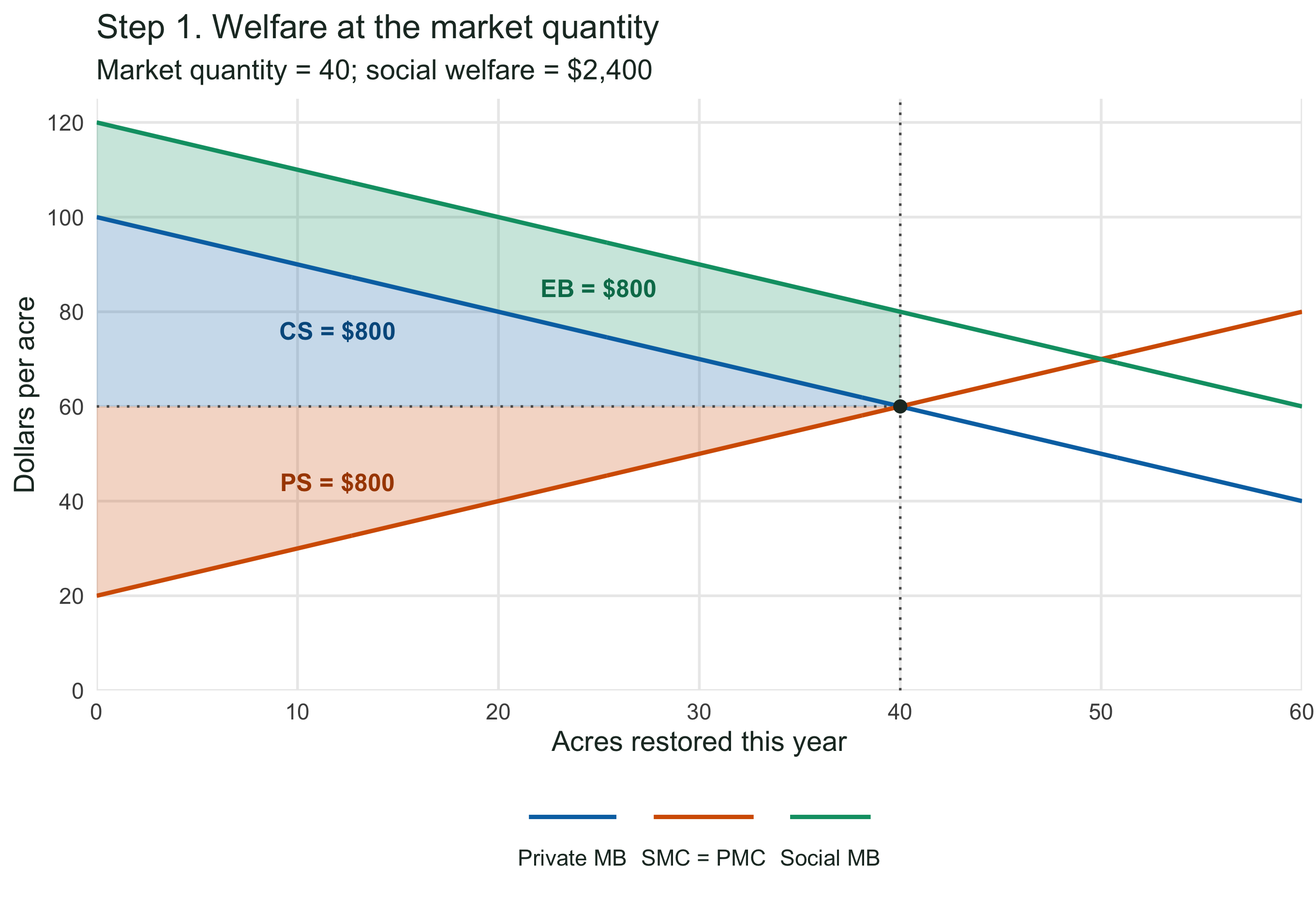
CS_M=\tfrac12(100-60)(40)=800,\qquad PS_M=\tfrac12(60-20)(40)=800,
EB_M=20(40)=800,\qquad SW_M=2{,}400.
With the subsidy:
CS_S=\tfrac12(100-50)(50)=1{,}250,\qquad PS_S=\tfrac12(70-20)(50)=1{,}250,
EB_S=20(50)=1{,}000,\qquad SW_S=1{,}250+1{,}250+1{,}000-1{,}000=2{,}500.
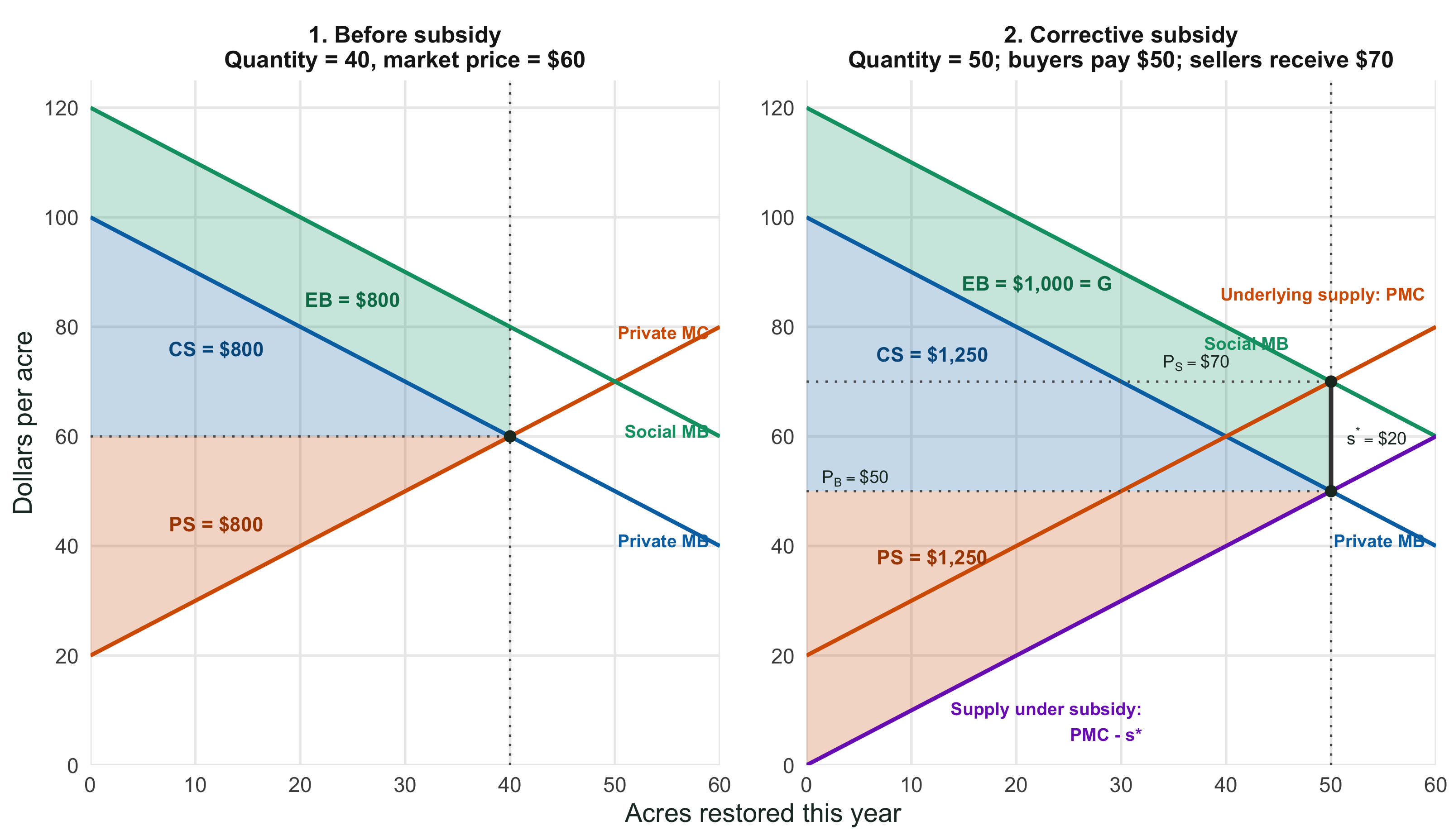
The purple line is the supply curve under the corrective subsidy. It lies 20 below the orange underlying supply curve because the government pays suppliers 20 for each restored acre. The subsidy does not lower the physical marginal cost of restoration; it lowers the amount buyers must pay to make each quantity worthwhile to suppliers.
At 50 acres, buyers pay 50 and suppliers receive 70 in total. The green area represents the $1,000 external benefit from those acres. Government subsidy spending is also $1,000 in this example. These values are equal here, but external benefits and government spending remain different concepts.
| Annual measure | Unregulated | Corrective subsidy |
|---|---|---|
| Consumer surplus | 800 | 1,250 |
| Producer surplus, including subsidy receipts | 800 | 1,250 |
| External benefits | 800 | 1,000 |
| Government spending | 0 | 1,000 |
| Social welfare | 2,400 | 2,500 |
The subsidy receipts benefit suppliers but are funded by others. Subtracting government spending offsets that transfer; otherwise the same public money would be counted as a new net social benefit. Under the exercise’s assumptions, the spending is not itself an additional real resource cost. Restoration’s real cost is already reflected by the supply curve.
(d) Graph (4 points)
Plot MB, SMB, and PMC. Mark both quantities and shade the welfare gain from correcting underprovision. Calculate the shaded area.
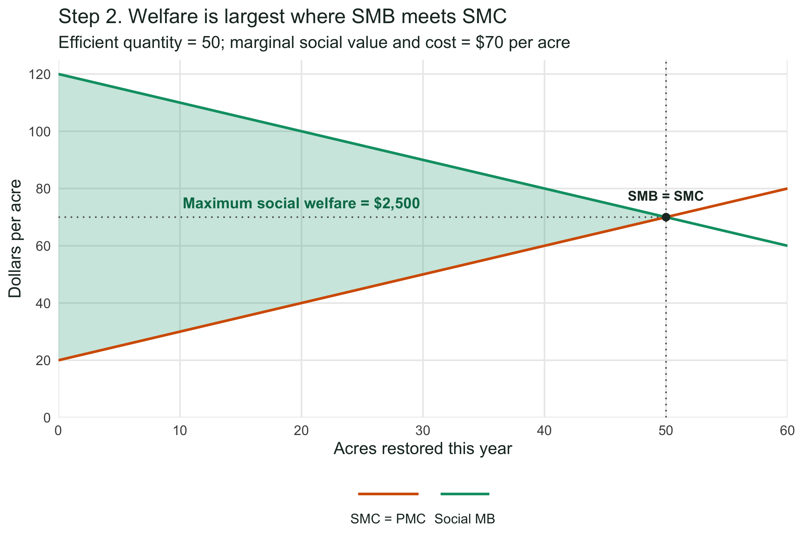
Compare social welfare at the market quantity with social welfare at the efficient quantity. In this problem, SMC=PMC because restoration creates an external benefit, not an external cost. At Q^*=50, SMB=SMC=70. The 70 is the marginal social value and marginal cost at the efficient quantity—not the price buyers pay under the subsidy. Buyers pay 50, while suppliers receive 70.
Step 1: Start from the market allocation
The first graph repeats the unregulated panel from part (c). At Q_M=40, the three shaded areas sum to social welfare of 2{,}400.
Step 2: Identify maximum social welfare
For society, each acre is worthwhile while SMB exceeds SMC. The curves meet at Q^*=50, so the entire shaded area through 50 acres is the maximum social welfare: 2{,}500.
Step 3: Isolate what the market leaves unrealized
The welfare through the first 40 acres is common to both outcomes. Once that common area is set aside, the only difference is the triangle between SMB and SMC from 40 to 50 acres.
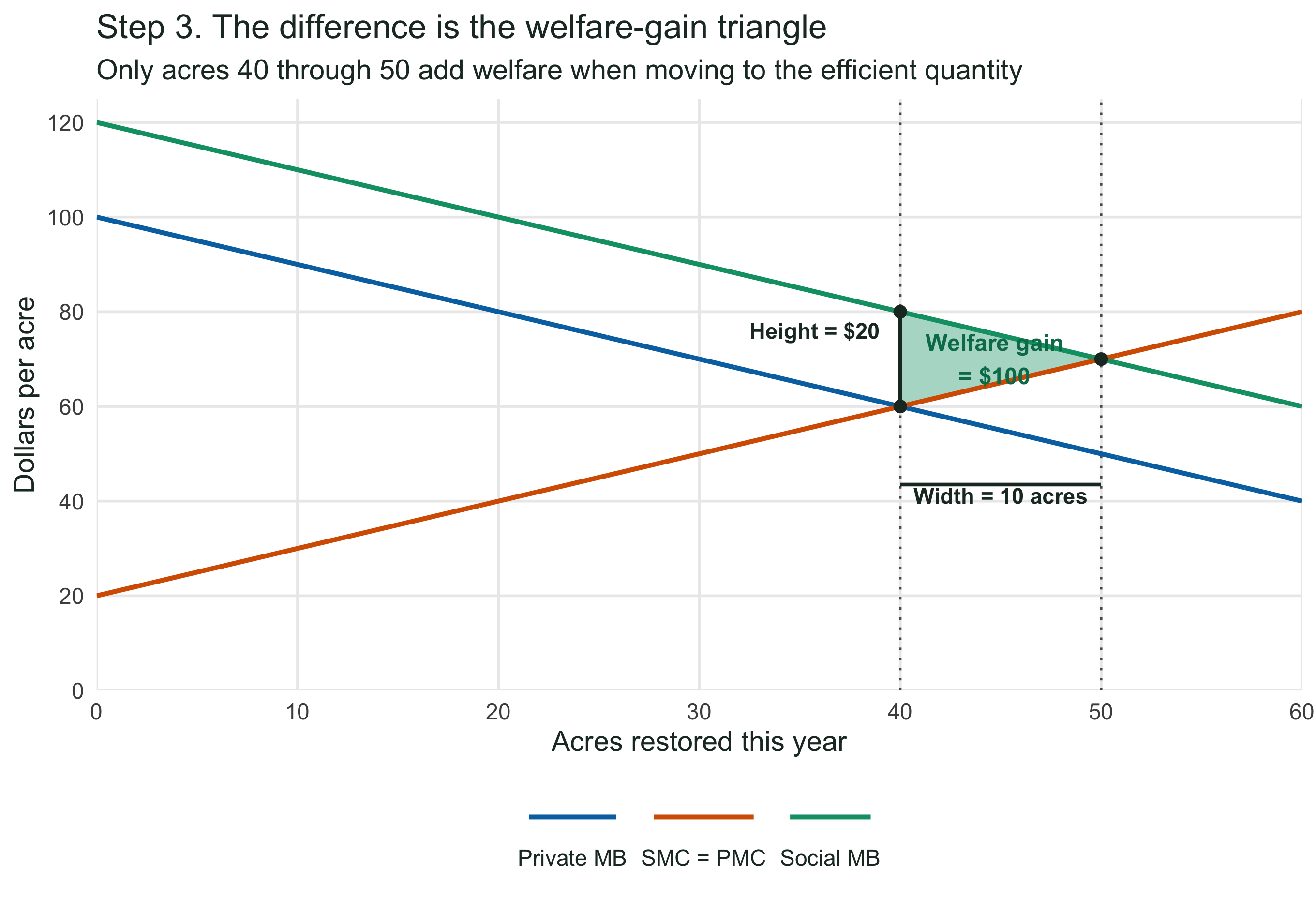
The same gain appears in both calculations:
SW(Q^*)-SW(Q_M)=2{,}500-2{,}400=100,
\Delta SW=\tfrac12(50-40)(80-60)=100.
(e) Policy design (5 points; 100–140 words)
Suppose two restored acres have very different downstream benefits. Explain why paying the same subsidy for every acre may not produce an efficient allocation. Identify one observable site characteristic that could help target payments, one outcome the agency should verify, and one reason it may be difficult to determine whether the credited improvement was caused by the subsidy.
2. Effort in an open-access fishery (25 points)

Consider the simplified total and marginal framework from Lecture 4. Let E be total seasonal fishing effort, measured in boat-days, with 0\leq E\leq120. Total catch revenue and total opportunity cost are
TB(E)=120E-E^2,\qquad TC(E)=20E.
For E>0, average benefit is AB(E)=120-E. The marginal schedules are supplied so that you do not need calculus:
MB(E)=120-2E,\qquad MC(E)=AC(E)=20.
Effort is divisible. In the open-access model, entrants expect the average revenue per boat-day and may enter freely. Costs include the opportunity cost of labor and equipment. For this exercise, the given revenue curve summarizes the resource constraints; do not add a separate damage curve or solve a dynamic stock model.
(a) Efficient effort (5 points)
Find E^*, total revenue, total cost, and economic rent TB-TC at the efficient outcome. Explain the marginal condition.
(b) Open-access effort (5 points)
Find the positive open-access equilibrium E_{OA}, total revenue, total cost, and economic rent. Explain why entry is governed by AB=AC, rather than MB=MC.
(c) Two-panel graph (6 points)
Draw TB and TC in a top panel, and AB, MB, and MC=AC in a bottom panel. Align the effort axes and mark E^* and E_{OA}. Calculate the rent lost under open access. Does zero economic rent mean that boats catch no fish or that fishers receive no income?
The efficient quantity maximizes the vertical gap TB-TC in the top panel and satisfies MB=MC below. The positive open-access outcome occurs where TB=TC and AB=AC.
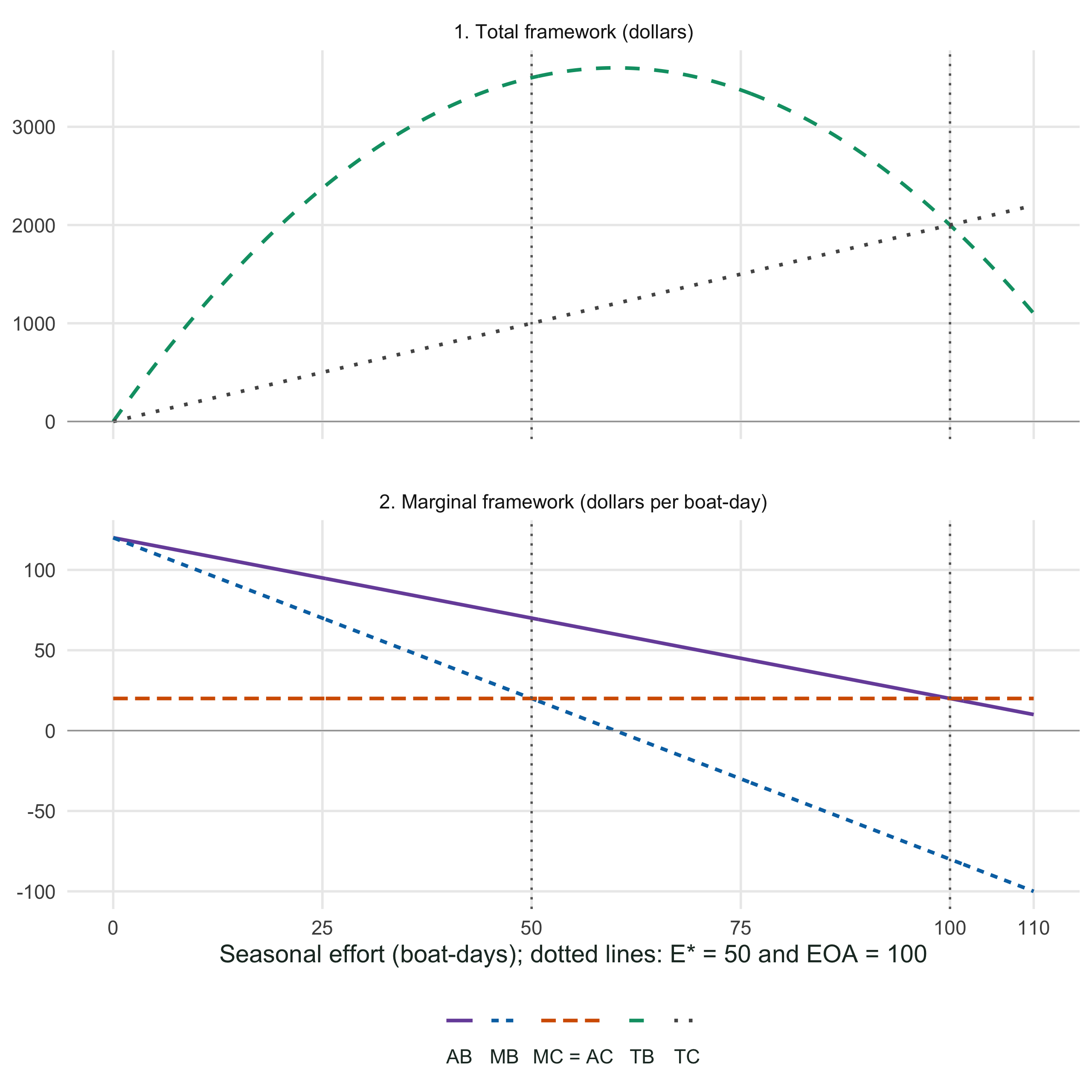
Open access loses 2{,}500 in rent. The lower panel gives the same result: between 50 and 100, MC-MB rises from 0 to 100, so \tfrac12(100-50)(100)=2{,}500. Zero economic rent means receipts cover opportunity costs, including labor and equipment. It does not mean zero catch or zero gross income. The model still has $2,000 in catch revenue at open access.
(d) Resource type and rules (4 points; 100–140 words)
Explain why a fish stock is a common-pool resource. Distinguish this physical characteristic from common property and open access. Would a defined community with enforceable access and effort rules necessarily reach E_{OA}? Explain.
(e) Costs through time (5 points; 100–140 words)
A boat’s wake damages a shoreline today, and its catch leaves fewer fish available for later use. Distinguish Lecture 3’s externality cost from stock-scarcity cost in these examples. Explain why secure ownership could make a user account for future scarcity, yet still leave harm to shoreline owners outside that user’s decision.
3. Lake Erie: algae, economic losses, and institutions (50 points)

Read Kaylee Wells’s Marketplace report, “How algae can crater Lake Erie’s economy” (July 6, 2026). The corresponding audio report appears in the July 6 episode, Back-to-school shopping? Already? A complete, lightly edited transcript of the Lake Erie report is provided below.
Transcribed from the supplied audio transcript and lightly edited for punctuation, speaker labels, and obvious automated-transcription errors.
Host (Kai Ryssdal): Every year, the National Oceanic and Atmospheric Administration predicts just how bad the algae are going to be on Lake Erie. The latest forecast is just out: a moderate harmful algal bloom is the estimate for the year. Those blooms are obviously a bummer for fish and for kids who want to go swimming, but they have massive economic implications, too, for people living nearby and for visitors. From the warm, slightly green waters of Lake Erie, Marketplace’s Kaylee Wells explains.
Reporter (Kaylee Wells): The blooms are a big enough deal that Lake Erie is dotted with little buoys constantly monitoring how much algae are in the water. It takes several minutes in a zippy speedboat to travel far enough offshore to see one up close. On the way, one of the scientists captures a jar full of water and holds it up to the light. It looks clear enough to drink. But then she throws a net with a filter on the end overboard and drags it through roughly a thousand gallons of water to reveal all the stuff we cannot see. The liquid remaining in the filter is murky, yellow-green, and scuzzy, with tiny zooplankton buzzing around and nipping at the green bits. In summer, the water temperature is near 70 degrees.
Scientist: We are certainly catching a lot of living stuff in the water.
Reporter: Ed Verhamme is our captain on today’s voyage. He is also a principal and senior engineer at LimnoTech, a consulting firm that helps make water cleaner.
Ed Verhamme: What we do not want is the harmful algae.
Reporter: That is the kind of algae that can cause diarrhea, vomiting, and rashes, and it is what his company helps monitor. Verhamme keeps driving until we arrive at a buoy. He pulls up the data it is capturing on his phone and relays the good news.
Ed Verhamme: Yep, really nothing going on out there right now, so these are very low readings.
Reporter: The recipe for high readings? Extremely heavy rainy periods, which pull nutrient-rich agricultural runoff into the lake, followed by extremely dry and sunny periods that help the algae form. This year has not been very extreme, which is why NOAA says it will be a moderate year for harmful algae. Verhamme says an especially bad year, like 2014, when algae contaminated Toledo’s water supply, would show readings 20 or 25 times higher than these, and the blooms would be very visible.
Ed Verhamme: That is noticeable scum. The water looks like paint, really.
Reporter: This year’s moderate forecast is not just good news for Lake Erie’s ecosystem. It means algae will not tank whole chunks of the Great Lakes economy this year. Lake Erie is the main source of drinking water for Northeast Ohio. Alex Margevicius, commissioner of Cleveland’s Water Division, says an algal bloom like the one in Toledo would be a doomsday scenario.
Alex Margevicius: I do not even know where to begin to calculate the economic impact of something like that. If greater Cleveland had to be under a do-not-drink-water advisory, what would happen?
Reporter: The background chatter comes from the State of the Great Lakes, an annual gathering of water experts and community members in downtown Cleveland. Clean water is a big deal here. The cost of algal blooms is calculated in more than bottled water and health-care bills.
Reporter: The $6 trillion economy of the Great Lakes Basin includes a huge tourism economy. Chris Ronayne is the executive of Cuyahoga County, which includes Cleveland.
Chris Ronayne: Lake Erie is the walleye capital of the world. People come here to fish. There are fishing tournaments and recreational anglers.
Reporter: When the algae get bad, they use up oxygen in the water, which causes mass fish kills—not an appealing feature in the walleye capital of the world. A hit to the tourism industry can have ripple effects, says Scott Hardy, an earth scientist with the Ohio State University.
Scott Hardy: That is not only going to affect the people who come to recreate. You have to think about the hotels where people stay. You have to think about the gas stations that fill the cars people drive to the water.
Reporter: Hardy says climate change is making the extreme weather, and the algal blooms that follow it, more common. But he also says we are getting better at mitigating the runoff that causes the blooms in the first place. Every year is therefore a toss-up in terms of how bad it will be. From the waters of Lake Erie, I am Kaylee Wells for Marketplace.
(a) Identify and explain the negative externality (8 points; 160–200 words)
Using Kaylee Wells’s Marketplace report, “How algae can crater Lake Erie’s economy”, the transcript provided above, and course terminology, explain why nutrient runoff associated with agricultural production is a negative production externality. Identify the private decision-maker and activity, at least two groups outside the market transaction that bear costs, and the external marginal cost (EMC) omitted from PMC. State how SMC, PMC, and EMC are related.
Using specific details, explain how nutrient loading creates the potential for harm, heavy rain transports nutrients into Lake Erie, and later dry, sunny weather affects bloom formation, timing, and severity. Conclude by explaining why an activity can be privately profitable but socially inefficient.
(b) Analyze rising marginal damage (10 points)
For parts (b)–(c), use this separate hypothetical watershed model. Q is units of agricultural output per season. Assume each unit creates one unit of nutrient runoff delivered to the lake, with no abatement option. The model is an illustration inspired by the reading, not an estimate reported by Marketplace:
MB(Q)=120-Q,\qquad PMC(Q)=20+Q,\qquad EMC(Q)=2Q.
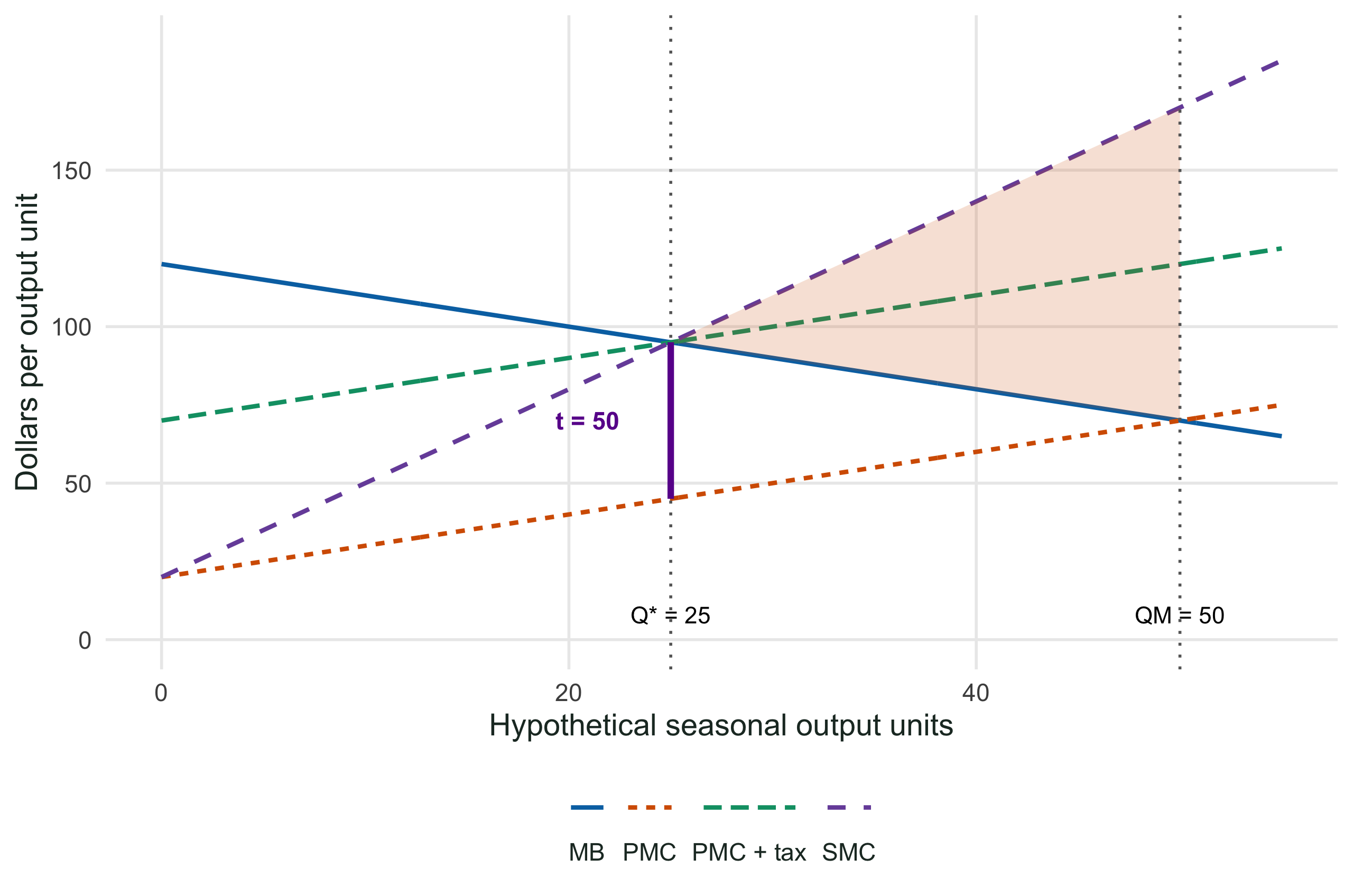
Find Q_M, write SMC(Q), and find Q^*. Calculate total external damage at each quantity using the area under EMC. Find the constant per-unit tax that implements Q^* and the prices buyers pay and suppliers retain under it. On one graph, draw MB, PMC, SMC, and the supply curve with the tax; mark Q_M, Q^*, and the tax wedge.
The unregulated market has
120-Q=20+Q\quad\Rightarrow\quad Q_M=50,\quad P_M=70.
Social cost and the efficient quantity are
SMC(Q)=20+Q+2Q=20+3Q,
120-Q=20+3Q\quad\Rightarrow\quad Q^*=25.
Total damage is the triangle under EMC(Q)=2Q:
ED(Q)=\tfrac12 Q(2Q)=Q^2.
Thus ED_M=50^2=2{,}500 and ED^*=25^2=625.
t^*=EMC(25)=50,\qquad P_B=MB(25)=95,\qquad P_S=PMC(25)=45.
The fixed per-unit tax shifts private supply to PMC+t^*=70+Q. This taxed supply intersects MB at Q=25. It is not identical to SMC=20+3Q at every quantity; the two curves coincide at the desired quantity.
(c) Account for welfare (10 points)
Calculate tax revenue and remaining external damage at Q^*. Are they equal? Explain why a Pigouvian tax need not equal total remaining damage when EMC rises with Q. Calculate the welfare gain using the deadweight-loss triangle. Then verify it by calculating CS, PS, tax revenue, external damage, and SW before and after the tax in a table.
(d) Classify information and the fishery (6 points; 120–160 words)
Case assumption: Suppose the buoy readings are posted online for anyone to use. Apply rivalry and excludability to classify the posted information. Contrast it with a walleye removed from the lake and explain why the fish stock is a common-pool resource. Finally, explain whether better public information alone gives upstream producers an incentive to include downstream runoff damage in their production decisions.
(e) Recommend an institution (10 points; 200–250 words)
Case assumptions: Nutrient runoff comes from many farms, individual contributions are not directly observed, and rainfall changes how much nutrient reaches the lake. Compare these three approaches:
- a charge on measured runoff;
- a required protective farming practice; and
- judicial liability for downstream harm.
For each approach, identify what must be measured or verified and who initially pays. Explain why lakewide buoy readings reveal lake conditions but do not identify each farm’s contribution. Recommend one approach as the main policy, state one important limitation, and explain why a tax on agricultural output becomes an imperfect substitute for a runoff charge when the assumed one-to-one relationship between output and runoff is relaxed.
(f) Interpret claims about economic losses (6 points; 130–170 words)
The report describes the Great Lakes Basin as a $6 trillion economy and notes possible effects on hotels and gas stations. Explain why $6 trillion is not an estimate of damage from a Lake Erie bloom. Explain why adding every affected firm’s lost sales could overstate welfare loss. Your answer must include examples to support your explanation.