Resource Allocation Over Time

A complete guide to nonrenewable-resource use across generations

A study guide to marginal net benefit, present value, user cost, depletion taxes, scarcity rent, Hotelling’s rule, the Hartwick rule, intertemporal fairness, and sustainability.

NoteFocus questions

1. How should a limited nonrenewable resource be divided across generations?
2. How can benefits and costs at different dates be compared?
3. How do scarcity, prices, and consumption change as a resource is depleted?
4. When is an efficient allocation also fair to future generations?

1. Renewable and nonrenewable resources

A renewable resource can regenerate through ecological processes. Farms, forests, and fisheries can remain productive for long periods when harvest does not continually exceed renewal. Renewable does not mean impossible to deplete.

A nonrenewable resource does not regenerate on a human time scale. Oil, coal, and mineral deposits are common examples. Extracting a unit today reduces the physical stock available later.

The economic question is not simply whether a nonrenewable stock will decline. The question is how to compare the value of using one more unit now with the value of preserving it for future use. Technology, substitution, new discoveries, and recycling can change effective scarcity, but they do not remove the need to make choices across time.

This guide studies recoverable neodymium in a known deposit using a two-period model. The model is deliberately simple. It reveals the main logic that carries into models with many periods.

2. The neodymium market in one period

Neodymium in this model

Illustration of a neodymium supply chain from a mineral deposit through separated material to a permanent-magnet motor.

Neodymium is a rare earth element used in high-strength permanent magnets. These magnets appear in electric motors and some wind-turbine generators. Rare earth elements are relatively abundant in Earth’s crust, but mineable concentrations are less common.

The model tracks 250 hypothetical tons of recoverable neodymium in one known deposit. Quantity measures recoverable neodymium content rather than the mass of raw ore. The supply curve includes marginal mining, separation, and processing cost.

Actual ores contain several rare earth elements that producers recover jointly. The model temporarily treats neodymium as a single product. Its equations and numerical values illustrate the economic logic rather than estimate the current neodymium market.

Supply, demand, and the static equilibrium

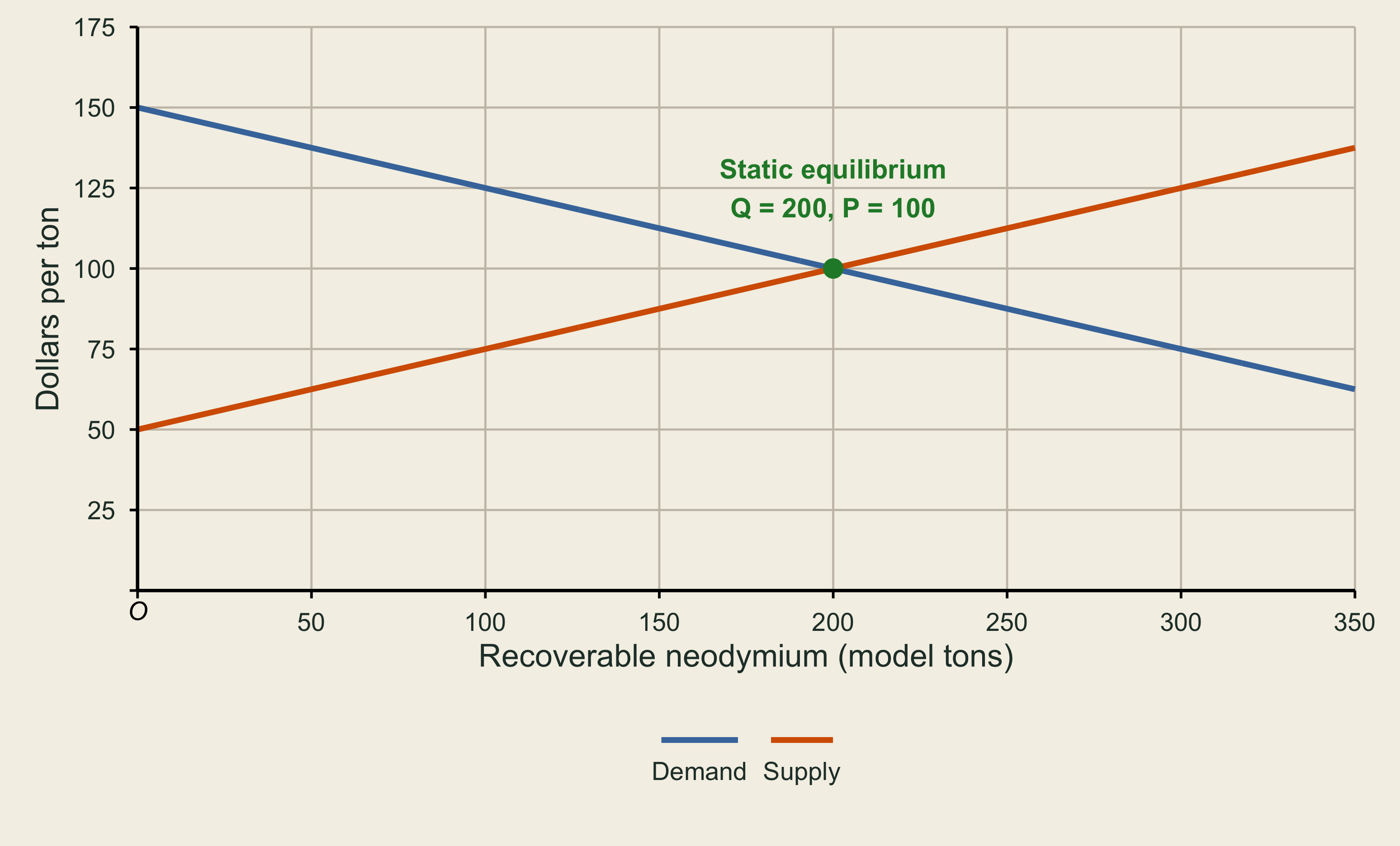
Suppose this illustrative neodymium market has these inverse demand and supply equations:

P_D=150-0.25Q,

P_S=50+0.25Q.

Demand measures permanent-magnet manufacturers’ marginal willingness to pay. Supply measures marginal mining, separation, and processing cost.

Setting the curves equal gives the one-period equilibrium:

150-0.25Q=50+0.25Q,

Q=200,\qquad P=100.

Figure 1: If only current benefits and costs matter, the illustrative neodymium market clears at 200 model tons and $100 per ton.

This is a static equilibrium because the calculation counts only benefits and costs in the current period.

Marginal net benefit

The marginal net benefit (MNB) of one more ton is its marginal benefit minus its marginal cost. It compresses the demand and supply information into one curve:

MNB=P_D-P_S.

For this market,

MNB=(150-0.25Q)-(50+0.25Q)=100-0.5Q.

At low quantities, buyers’ willingness to pay substantially exceeds extraction cost. MNB falls as quantity increases. It reaches zero at Q=200, where the market reaches its static equilibrium. Production beyond 200 would have negative marginal net benefit.

Figure 2: The area under MNB through 200 model tons is the total net benefit of the illustrative neodymium market.

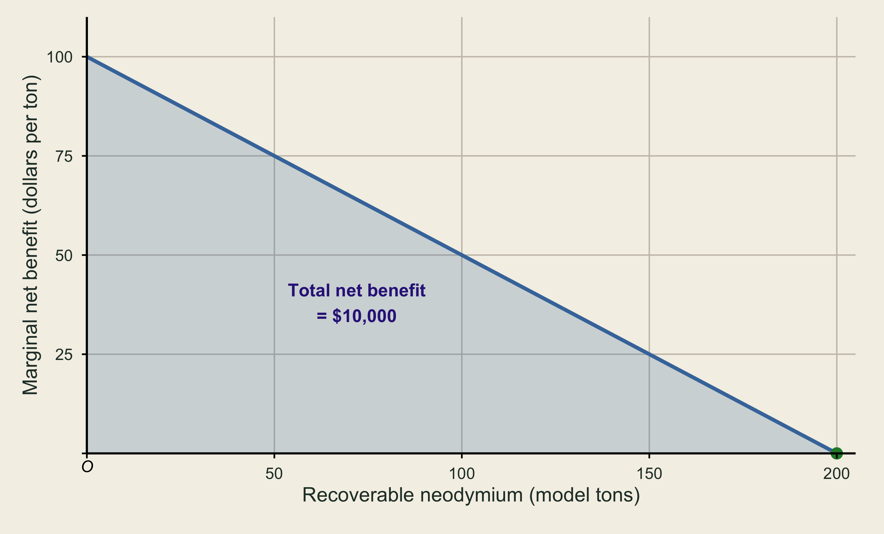
The area under MNB is total net benefit, which equals total benefit minus total cost. Here it is the area of a triangle:

TNB=\frac12(200)(100)=10{,}000.

Total net benefit reaches its maximum when MNB reaches zero. This reproduces the one-period market equilibrium.

3. A fixed stock across two periods

Suppose 250 model tons of recoverable neodymium must be divided between Period 1 and Period 2:

Q_1+Q_2=250.

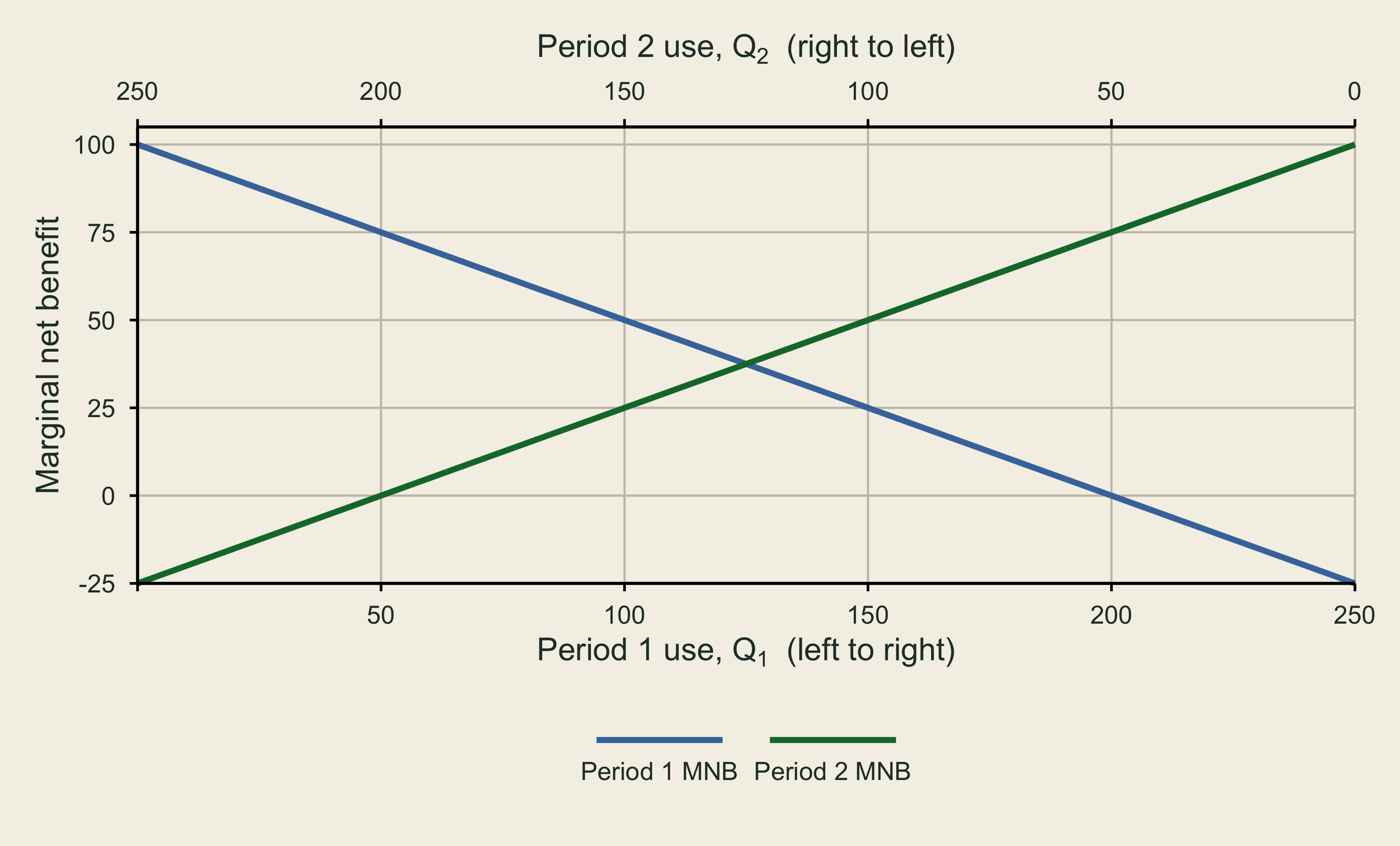
This supply constraint means that additional use in one period leaves exactly that much less for the other period. Assume that the demand, supply, and MNB functions are initially the same in both periods:

MNB_1=100-0.5Q_1,

MNB_2=100-0.5Q_2.

The mirror-axis graph reads Q_1 from left to right and Q_2 from right to left. Every point on the horizontal axis allocates all 250 tons.

Figure 3: The mirror axis keeps the 250-ton supply constraint visible: moving right increases Period 1 use and reduces Period 2 use by the same amount.

4. Present value and discounting

Present value converts a future benefit or cost into its value at a common earlier date. With annual discount rate r and n years between dates,

PV(X_n)=\frac{X_n}{(1+r)^n}.

The example uses a 7.25% annual rate and periods ten years apart. Five hundred dollars invested today at roughly 7.25% grows to about $1,000 after ten years. Equivalently, the present value of $1,000 received with certainty in ten years is about $500:

\frac{1{,}000}{(1.0725)^{10}}\approx 500.

The example assumes a real interest rate, meaning that expected inflation has already been removed. A person who prefers current cash could borrow against the certain future payment. That borrowing interpretation explains why two dated amounts can be economically equivalent.

For the neodymium example, the ten-year discount factor is approximately two:

PV[MNB_2]=\frac{MNB_2}{(1.0725)^{10}}\approx\frac{MNB_2}{2}.

Discounting therefore halves every Period 2 marginal net benefit when measured in Period 1 dollars.

5. Dynamic equilibrium

The efficient allocation makes Period 1 MNB equal to the present value of Period 2 MNB:

MNB_1=PV[MNB_2].

Together with the stock constraint, the model has two equations:

100-0.5Q_1=\frac{100-0.5Q_2}{2},

Q_1+Q_2=250.

Substituting Q_2=250-Q_1 gives

100-0.5Q_1=50-0.25(250-Q_1),

0.75Q_1=112.5,

Q_1=150,\qquad Q_2=100.

Figure 4: Figure 5.4 concept. At 150 tons now and 100 tons later, the marginal net benefits are equal after discounting, and combined discounted net benefit is maximized.

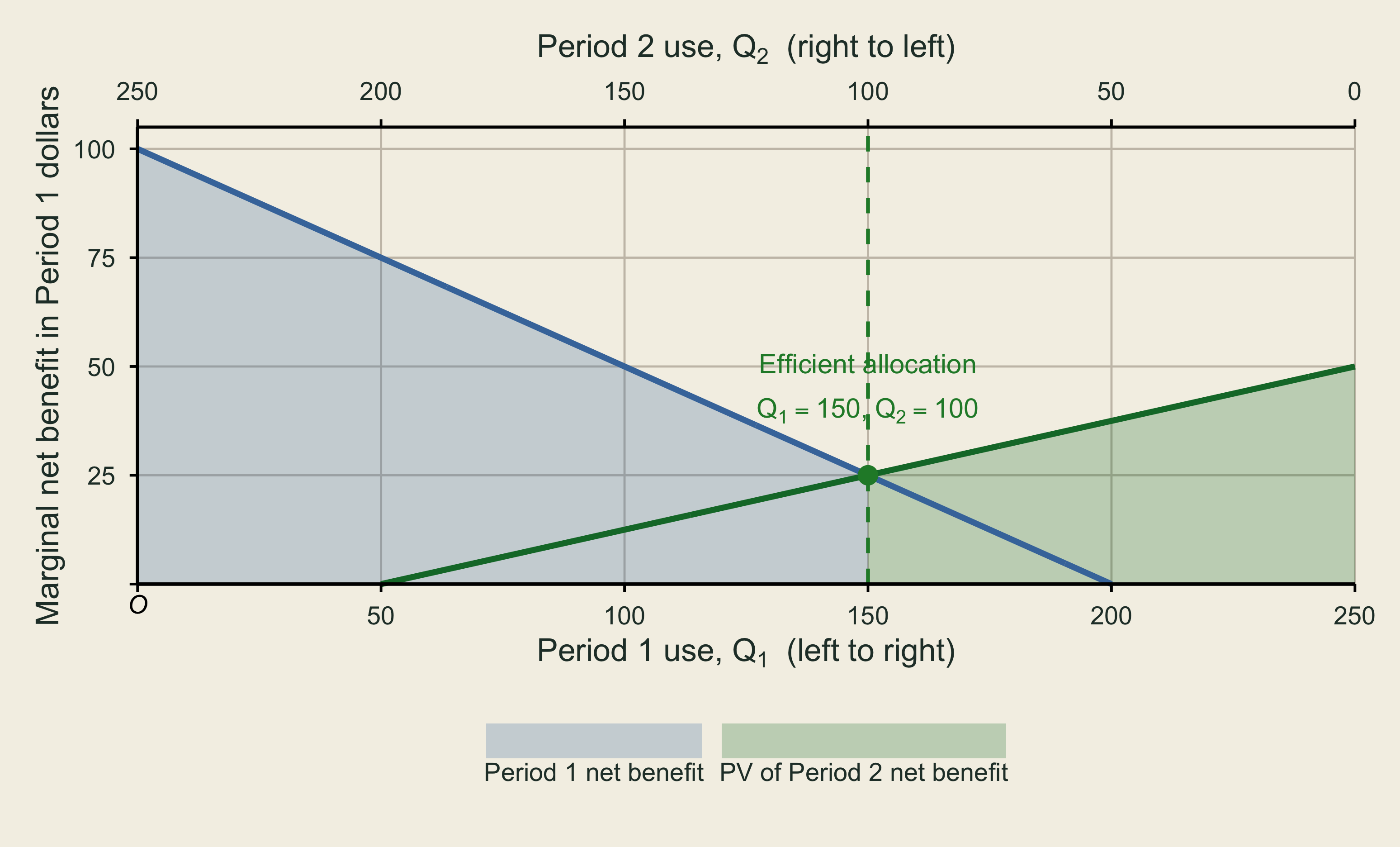
A dynamic equilibrium counts both present and future benefits and costs. The crossing maximizes the sum of Period 1 net benefit and the present value of Period 2 net benefit.

Why another allocation loses welfare

Consider Q_1=200 and Q_2=50. Shifting 50 tons from Period 2 to Period 1 adds some current net benefit, but the discounted future benefit lost is larger. The difference is a welfare loss.

Figure 5: Figure 5.5 concept. Moving from the efficient allocation to 200 tons in Period 1 sacrifices more discounted future benefit than it adds in current benefit.

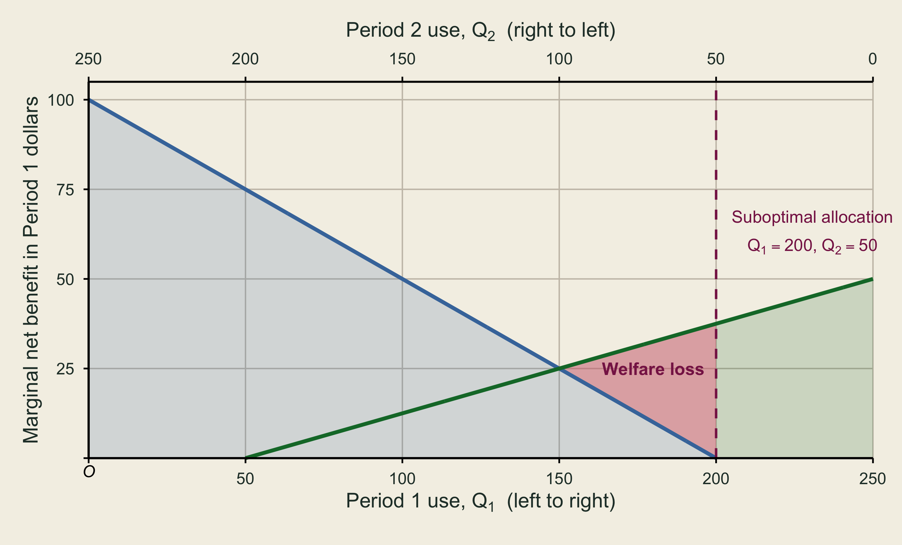
The opposite shift, such as Q_1=100 and Q_2=150, also moves away from the crossing and lowers discounted total net benefit.

6. User cost

Using a resource today can reduce the benefit available to future users. The lost future opportunity is the user cost of current extraction.

In this example, Period 2 would use at most 200 tons in its static market. If Period 1 uses no more than 50 tons, at least 200 remain, so one more current ton does not yet reduce the desired Period 2 quantity. Beyond 50 tons today, each additional current ton displaces a future ton. Its present-value loss appears as the rising PV[MNB_2] curve.

At the efficient allocation,

\text{User cost}=MNB_1(150)=100-0.5(150)=25,

and the same value appears from the future side:

\text{User cost}=PV[MNB_2(100)]=\frac{100-0.5(100)}{2}=25.

This framework describes user cost as an externality across time when the current market leaves the future loss out of current decisions. It also explains that forward-looking owners may anticipate scarcity and incorporate some or all of that value themselves.

Evidence from Jordan

ImportantEstimating user costs in Jordan

Jordan exports phosphate and potash used in fertilizer. A study of extraction from 2002 through 2010 estimated user costs of about $550 million using a 3% discount rate, roughly 20% of mining profits during the period.

The central sustainability issue was what happened to those proceeds. Using depletion income mainly for current consumption would leave fewer assets for future generations. Reinvesting the user-cost portion in education and skills, produced capital, or renewable natural capital could preserve a future income stream. The case therefore links measurement of user cost with governance and reinvestment.

The source note in the textbook attributes the estimate to Alrawashdeh and Al-Tarawneh (2014). The surrounding discussion gives a different publication year, so the primary source should be checked before citing its year independently.

7. Resource depletion policy

Social cost and the depletion tax

If the current market ignores user cost, it chooses 200 tons. Adding marginal user cost to extraction cost creates a social-cost schedule. A resource depletion tax can reproduce the efficient outcome when it equals the marginal user cost at the target quantity.

At Q_1=150, the correct tax is $25 per ton. The tax shifts the buyer-facing supply curve to

P=75+0.25Q.

Equating it with demand gives

150-0.25Q=75+0.25Q,

Q_1=150,\qquad P_1=112.50.

Figure 6: Figure 5.6 concept. User cost raises the full social cost of current extraction. A $25 depletion tax reaches the efficient Period 1 quantity of 150 tons.

The social-cost curve and the constant tax-adjusted supply curve differ away from the efficient quantity. They coincide at the efficient quantity because the tax equals marginal user cost there.

The second-period outcome

With 150 tons used in Period 1, 100 remain for Period 2. The demand curve gives

P_2=150-0.25(100)=125.

Figure 7: Figure 5.7 concept. The remaining stock fixes second-period supply at 100 tons, and demand determines a price of $125.

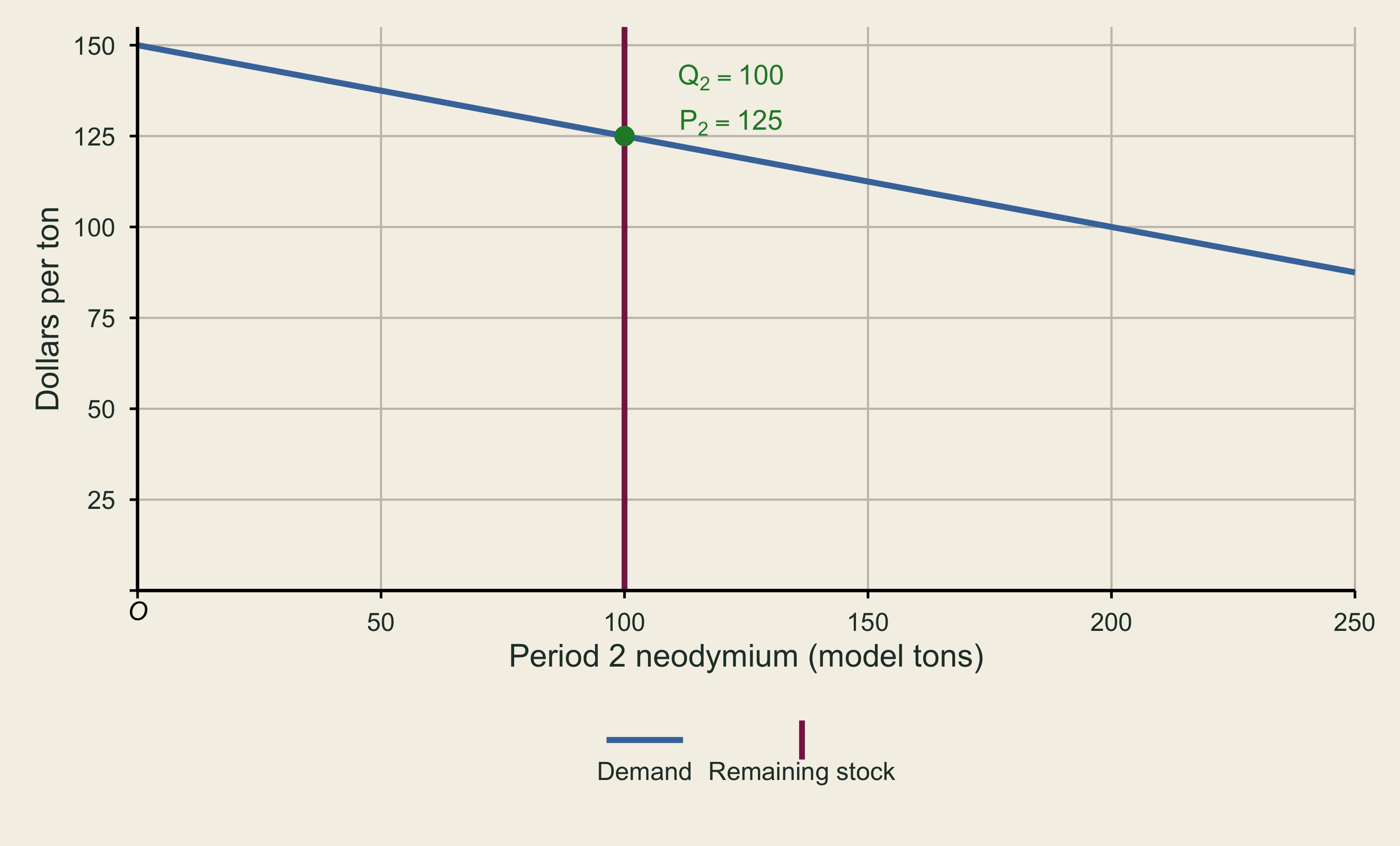
The higher current price discourages some present use and preserves more neodymium for the future. Other possible policies include direct limits on extraction, setting deposits aside, or maintaining public stockpiles of processed material.

8. Scarcity rent and private owners

Government intervention may be unnecessary when private owners can foresee scarcity, control extraction, and capture the future value of leaving resources underground.

To see the incentive, consider the static allocation of 200 tons now and 50 tons later. At 50 tons in Period 2,

P_D(50)=137.50,

P_S(50)=62.50.

The $75 difference is scarcity rent on the marginal unit:

137.50-62.50=75.

Scarcity rent is the payment above the amount needed to cover the marginal production cost. A forward-looking owner may withhold some current supply to earn larger discounted rent later. Under restrictive assumptions, profit maximization can produce the same two-period allocation as the depletion tax by equalizing discounted scarcity rents.

Reasons for caution remain. Owners may have short horizons, uncertain information, insecure claims, limited access to finance, or incentives that differ from social objectives. The relevant question is whether current market prices already contain the future scarcity value.

9. Discount rates change the allocation

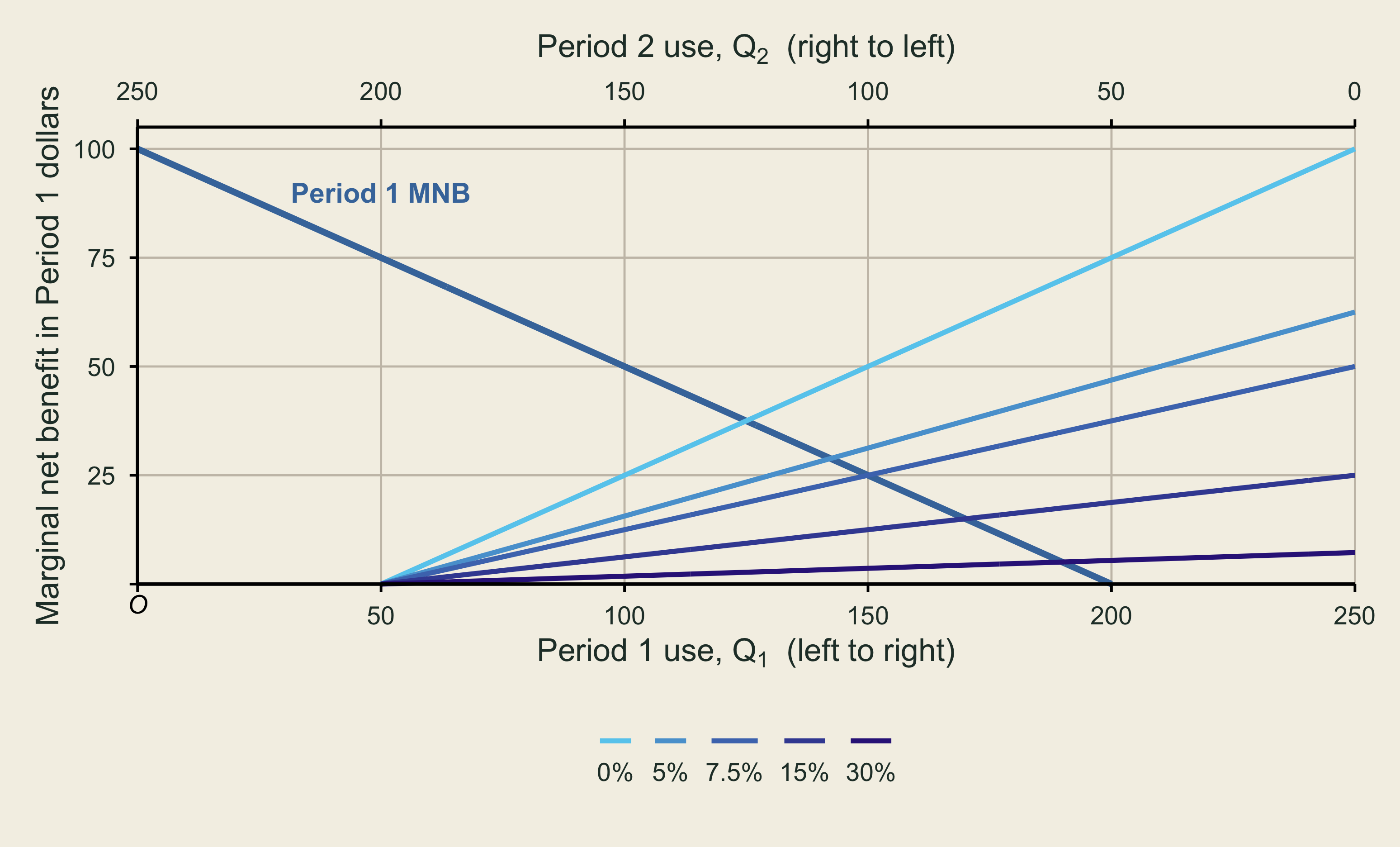
With a zero discount rate, the two periods receive equal weight and the stock divides evenly: 125 tons in each period. A positive discount rate gives more weight to current benefits. As the rate rises, the efficient allocation shifts toward Period 1 and user cost falls.

Figure 8: Figure 5.8 concept. Larger discount factors rotate the present-value curve downward, moving the crossing toward greater Period 1 use.

Annual discount rate	Ten-year factor, (1+r)^{10}	Q_1	Q_2
0%	1.0	125	125
2%	1.2	132	118
5%	1.6	143	107
7.5%	2.0	150	100
10%	2.6	158	92
15%	4.0	170	80
20%	6.2	179	71
30%	13.8	190	60

At 30%, the allocation approaches the static quantity of 200 tons in Period 1 and the user cost becomes small. Discounting over very long horizons can make distant benefits carry little present weight.

10. Hotelling’s rule

The two-period logic extends to many dates. Hotelling’s rule states that, in equilibrium, the net price of a nonrenewable resource rises at the interest rate:

R_{t+1}=(1+r)R_t,

where R_t, the net price or scarcity rent, is market price minus marginal extraction cost in year t, and r is the market interest rate.

The owner’s choice explains the rule:

• If current rent invested at interest would exceed expected future rent, extracting now pays more.
• If expected future rent would exceed current rent plus interest, waiting pays more.
• Extraction adjusts until the owner is indifferent at the margin.

With an initial net price of 100 and a 7% rate,

R_t=100(1.07)^t.

Figure 9: Figure 5.9 concept. In the benchmark, net price follows an exponential path whose growth rate equals the interest rate.

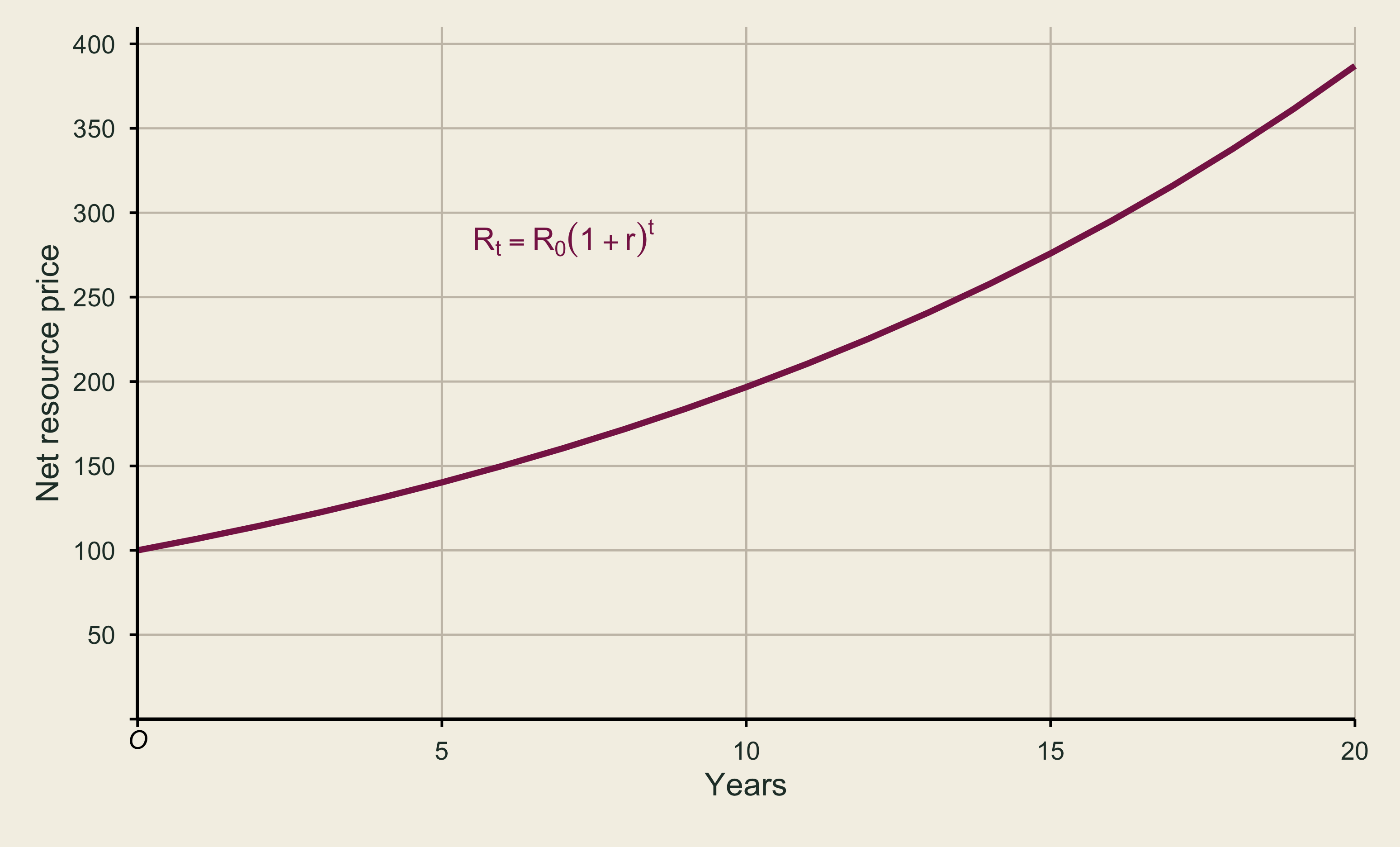
Higher interest rates encourage faster extraction because earning a market return on current proceeds becomes more attractive. Economic theory therefore implies an optimal depletion rate that maximizes the resource’s net present value. Under the benchmark assumptions, complete exhaustion can be part of that optimum.

Observed resource prices need not follow a smooth Hotelling path. New discoveries, technical change, changing extraction costs, market power, taxes, uncertainty, environmental policy, substitution, and recycling can all alter the observed price.

11. The Hartwick rule and future generations

Complete physical depletion raises an ethical question. The Hartwick rule distinguishes conserving a particular deposit from preserving productive capacity for future people. It says that society should invest scarcity rents from nonrenewable extraction rather than consume them:

\text{scarcity rent}=\text{resource revenue}-\text{extraction cost}.

NoteNatural capital

Natural capital is the stock of natural resources and ecosystems that generates benefits over time. For example, a standing forest is natural capital because it can provide timber while also storing carbon, regulating water flows, and supporting wildlife habitat.

Investment in skills, infrastructure, technology, or renewable natural capital can leave future generations other productive assets. This is a weak-sustainability argument because it permits produced capital to replace depleted natural capital.

A key limitation is that produced assets may not adequately replace natural capital with unique ecological, cultural, or life-support functions. The substitution argument is more plausible for a mineral deposit with little separate ecological value than for a critical ecosystem.

12. Limits and extensions

Discounting and distant generations

A market interest rate can place very little weight on effects far in the future. That raises a normative question: should commercial returns determine how society values the welfare of distant generations? Cost-benefit analysis often distinguishes a social discount rate from private market returns because the choice contains ethical as well as financial judgments.

Environmental externalities

The basic neodymium model assumes that the supply curve captures all social extraction costs. Mining, ore concentration, and chemical separation can affect water, landscapes, habitat, and human health while generating tailings and other wastes. Adding those costs would change the efficient price and extraction path.

Recycling and additional supply

The model also omits recycling. Recovering neodymium from manufacturing scrap or end-of-life permanent magnets can add secondary supply and reduce pressure on newly mined deposits. New discoveries and technical change can similarly expand economically recoverable supply. These extensions alter the numerical path without removing the intertemporal logic.

Assumptions behind the model

• Rare earth elements are relatively abundant in Earth’s crust, but mineable concentrations are less common.
• The 250-ton stock represents hypothetical recoverable neodymium content rather than raw ore mass or a measured real-world reserve.
• The model initially ignores joint production with other rare earth elements, recycling, substitution, and new discoveries.
• Periods are ten years apart, and all remaining stock is used by Period 2.
• Supply and demand functions are unchanged between periods.
• The 7.25% rate is real rather than nominal.
• The benchmark initially omits environmental externalities.
• Hotelling’s rule originates with Harold Hotelling’s 1931 analysis and has mixed empirical performance for observed commodity prices.

Further reading and source notes

• Later portions of the source text develop recycling, add extraction externalities, and examine evidence on resource prices and extraction.
• The investment rule is traced to Hartwick (1977) and Solow (1986).

13. Summary

1. A nonrenewable stock used today cannot also be used later. Efficient allocation compares current marginal net benefit with the present value of the future marginal net benefit forgone.
2. Present value places dated benefits and costs on one clock. A higher discount rate shifts more use toward the present.
3. The illustrative one-period neodymium market selects 200 model tons. With a 250-ton stock and a ten-year discount factor of two, the dynamic allocation is 150 tons now and 100 tons later.
4. User cost measures the lost future opportunity created by current extraction. At the efficient Period 1 quantity, it is $25 per ton.
5. A $25 resource depletion tax can internalize this user cost, raising the Period 1 price to $112.50 and reducing current use to 150 tons.
6. Forward-looking owners may capitalize scarcity into prices. Scarcity rent gives them an incentive to withhold some current supply.
7. Hotelling’s rule says the net resource price rises at the interest rate in the benchmark model. Higher rates imply faster depletion.
8. The Hartwick rule directs scarcity rents into investment for future well-being, but its adequacy depends on whether other capital can substitute for the depleted natural asset.
9. Long-horizon discounting, environmental damage, uncertainty, market imperfections, recycling, substitution, discovery, and technical change limit the simple model.

14. Key terms

Term	Meaning here
Renewable resource	A resource regenerated through ecological processes, although excessive use can still deplete it
Nonrenewable resource	A resource that does not regenerate on a human time scale
Recoverable neodymium	Neodymium content in a known deposit that can be produced under the model’s assumed technology and costs
Marginal net benefit	Marginal benefit minus marginal cost for one more unit
Total net benefit	Total benefit minus total cost, represented by the area under MNB
Static equilibrium	An equilibrium based only on current benefits and costs
Present value	A future value expressed in current-value terms
Discount rate	The rate used to translate future benefits and costs into present values
Supply constraint	The fixed total stock that must be allocated across dates
Dynamic equilibrium	An equilibrium that counts present and future benefits and costs
User cost	The opportunity cost of future use lost through current extraction
Social cost	Market and nonmarket costs associated with a good or service
Resource depletion tax	A tax on extraction or sale designed to reflect user cost
Scarcity rent	The resource price net of the marginal cost needed to supply it
Hotelling’s rule	The benchmark condition that net resource price rises at the interest rate
Optimal depletion rate	The extraction path that maximizes the resource’s net present value
Hartwick rule	The principle that scarcity rents should be invested rather than consumed

15. Discussion questions

1. Private traders may anticipate scarcity and conserve a resource for future profit. Under what conditions is that argument convincing? When might public policy improve the outcome, and which policy tool would fit the problem?
2. Can this framework be applied to the atmosphere or oceans? Identify where a fixed-stock model helps and where regeneration, common access, ecosystem thresholds, or pollution make its conclusions incomplete.

16. Defining intertemporal fairness

Efficiency and fairness are different standards. Efficiency is mainly concerned with eliminating waste in the use of resources. Fairness is concerned with the treatment of all affected parties, including people who are not yet born. No single standard of fairness is universally accepted, but one standard with prominent support concerns the legacy that earlier generations leave to later ones.

Intergenerational fairness is particularly difficult because future generations cannot speak for themselves, let alone bargain with the people alive today. No one alive in a later period can offer to accept radioactive waste in exchange for plentiful supplies of titanium.

The veil of ignorance

The philosopher John Rawls proposed a thought experiment for deriving principles of justice. People choose the rules for their society in an “original position,” behind a veil of ignorance that hides where they will end up in that society, and they must then live under whatever rules they chose.

Across time, picture every generation, present and future, choosing together the rules that will divide resources among them. Because no participant knows which generation they will join, the rules they choose would be neither excessively conservationist, which would hurt them if they were born early, nor excessively exploitative, which would hurt them if they were born late.

The sustainability criterion

One rule that could emerge from such a meeting is the sustainability criterion.

NoteSustainability criterion

“At a minimum, future generations should be left no worse off than current generations” (Tietenberg and Lewis 2023, p. 120). Making later generations poorer so that earlier ones can be richer fails the test.

The criterion does not prohibit using depletable resources. Earlier generations may use resources that later generations will therefore not have, as long as the well-being of later generations remains at least as high as that of earlier generations. It is violated only when current use pushes future well-being below the level that earlier generations enjoyed.

This definition leads to a practical question: do efficient allocations, or the institutions that produce them, adequately protect future generations?

17. Are efficient allocations fair?

The efficient allocation without sharing

The neodymium model offers a direct test. Measure each period’s net benefit in that period’s own dollars, without discounting, because the sustainability criterion compares the well-being of the people living in each period. Net benefit in a period is the area under that period’s MNB curve up to the quantity used there. For Q\le200, the area is a trapezoid:

NB(Q)=\frac{Q\,[100+MNB(Q)]}{2}=100Q-0.25Q^2.

Compare the dynamic efficient allocation with an allocation that divides the 250 tons equally between the periods:

Allocation	Q_1	Q_2	Period 1 net benefit	Period 2 net benefit
Equal split	125	125	$8,593.75	$8,593.75
Efficient, no sharing	150	100	$9,375.00	$7,500.00

The efficient allocation gives more of the resource, and more net benefit, to Period 1. Without sharing, Period 2 receives $7,500, less than Period 1’s $9,375 and less than the $8,593.75 it would receive from an equal split. On its own, the efficient extraction path therefore violates the sustainability criterion.

Efficiency with sharing

Choosing the efficient extraction path does not prevent Period 1 from saving part of its net benefit for Period 2. Suppose Period 1 keeps $8,593.75, exactly what it would receive from an equal split, and invests the remaining

9{,}375-8{,}593.75=781.25.

At the model’s real interest rate, an investment doubles over the ten years between periods, which is the same factor of two used to discount Period 2 benefits. The savings therefore grow to

2\times781.25=1{,}562.50,

and Period 2 receives

7{,}500+1{,}562.50=9{,}062.50>8{,}593.75.

Period 1 is exactly as well off as under an equal split, and Period 2 is $468.75 better off. Period 2 now receives more than Period 1, so the sustainability criterion is satisfied. The argument depends on the savings earning a real return: the $781.25 must grow by a factor of at least 1.4, about 3.4% a year, for Period 2 to reach Period 1’s $8,593.75.

Figure 10: Tietenberg and Lewis’s sharing argument applied to the neodymium model. Without sharing, the efficient allocation leaves Period 2 below the equal-split benchmark. If Period 1 keeps its equal-split amount and invests the extra $781.25, Period 2 receives $9,062.50.

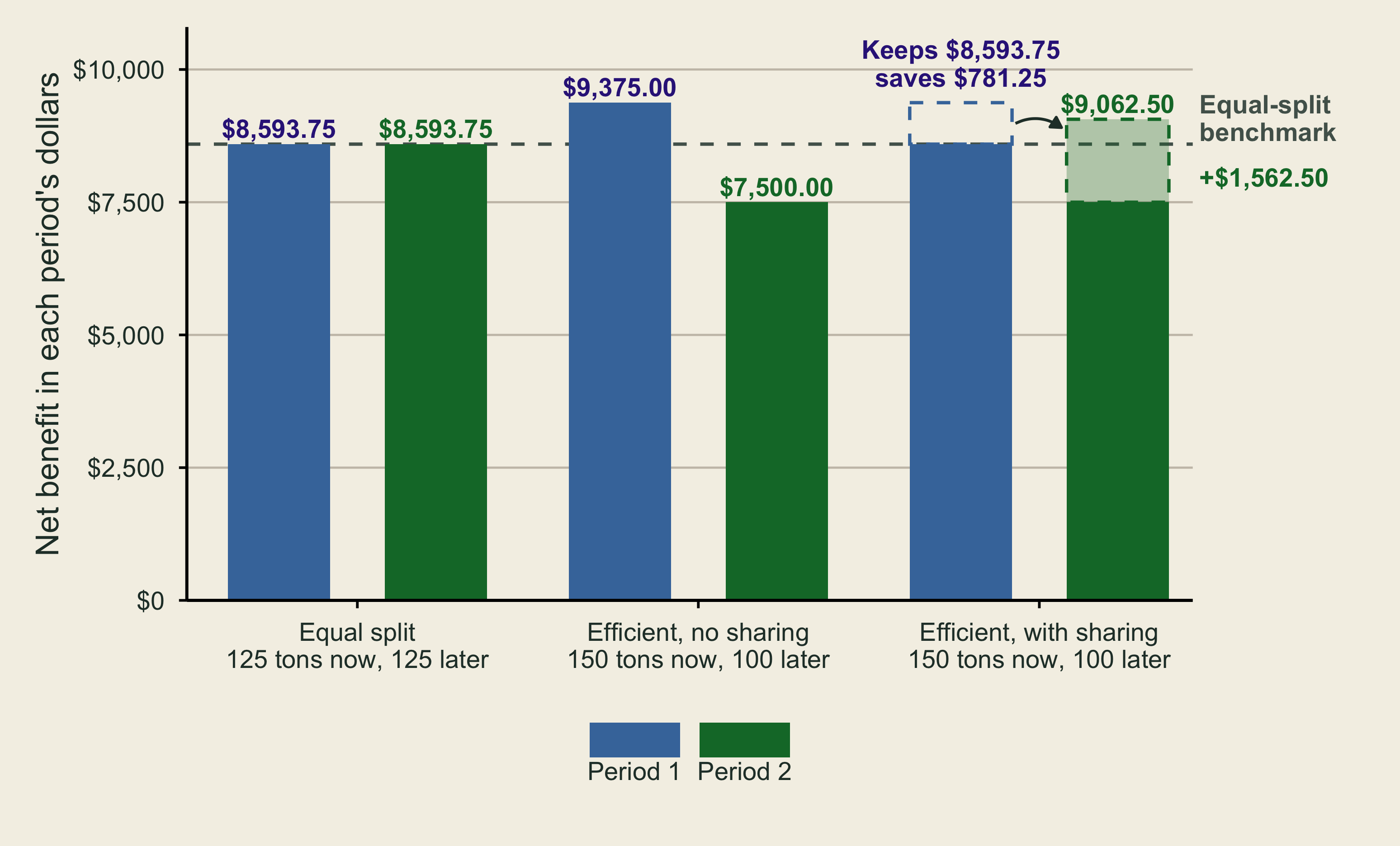
Sharing is possible because the efficient allocation creates more wealth to share. In Period 1 dollars, the efficient allocation yields 9{,}375+7{,}500/2=13{,}125 in discounted net benefit, while the equal split yields 8{,}593.75+8{,}593.75/2=12{,}890.625. The difference, $234.375 in Period 1 dollars, is worth 2\times234.375=468.75 dollars by Period 2, exactly Period 2’s gain in the sharing arrangement. The same logic holds generally: because a dynamically efficient allocation maximizes the present value of net benefits, enough of the first period’s gains can always be set aside to leave both periods at least as well off as under any other extraction path.

Tietenberg and Lewis make the same argument with a different numerical model. There, an equal split gives each period $40, while the efficient allocation gives $40.466 to the first period and $39.512 to the second. If the first period keeps $40 and saves $0.466 at 10% interest, the second period receives $39.512 + $0.513 = $40.025.

The lesson is conditional. An efficient allocation need not pass the sustainability test on its own, yet it can pass once sharing is added, even when the economy depends heavily on depletable resources. Nothing guarantees that the sharing happens, and Tietenberg and Lewis expect it to be the exception rather than the norm.

Example: the Alaska Permanent Fund

ImportantAn intergenerational sharing mechanism in Alaska

The Trans-Alaska Pipeline. Photo: Luca Galuzzi, 2005, CC BY-SA 2.5, via Wikimedia Commons.

Alaska’s oil fields generate large revenues, but every barrel pumped also draws down one of the state’s main natural assets. In 1976, with the trans-Alaska pipeline nearly finished, voters amended the state constitution to create the Alaska Permanent Fund, which sets aside part of the oil rents for future Alaskans.

The amendment requires that at least 25% of mineral lease rentals, royalties, royalty sale proceeds, federal mineral revenue-sharing payments, and bonuses received by the state be placed in a permanent fund whose principal may be used only for income-producing investments. State law later raised the deposit to 50% for leases issued after December 1, 1979. Spending the principal on current expenses would require a majority vote of Alaskans.

The fund is invested in a diversified portfolio that earns interest, dividends, rents, and capital gains. The legislature has used part of the annual earnings to pay a dividend to every eligible Alaska resident and has retained the rest so that inflation does not erode the endowment. As of December 2022, the fund’s market value was $74.46 billion, and the 2022 payment was $3,284 per resident: a $2,622 dividend plus a one-time $662 energy relief payment.

The fund preserves some revenue for future generations, but it falls short of full sustainability for two reasons. First, a majority of current voters could agree to spend the principal. The idea has been debated, although it has not happened. Second, only part of the revenue enters the fund: 25% of royalties from older leases and 50% from newer ones. If net revenue reflects scarcity rent, full sustainability would require investing all of it. Meanwhile, the current generation receives both its share of fund income and the rest of the proceeds from current oil sales.

Source: Tietenberg and Lewis (2023), Example 5.1, drawing on the Alaska Permanent Fund Corporation (apfc.org) and the Permanent Fund Dividend Division (pfd.alaska.gov), accessed January 19, 2023. The 50% deposit rate and the 2022 payment breakdown are from APFC and the Anchorage Daily News.

18. Applying the sustainability criterion

The Hartwick rule as an operational test

The sustainability criterion is difficult to apply directly. Determining whether future well-being will be lower than current well-being requires knowledge of future resource allocations and of future generations’ preferences, because those preferences determine how valuable different resource streams will be to them.

The Hartwick rule, introduced in Section 11, provides a more operational version. Hartwick (1977) showed that if all the scarcity rent from an exhaustible resource is invested in capital, consumption can be held constant forever, because the investment keeps the value of the total capital stock from falling.

This reinterpretation offers two insights:

1. An observable test. A decline in the value of the total capital stock signals an unsustainable path. The test can be run each year without forecasting future allocations or preferences, although valuing natural capital still requires prices that reflect expected scarcity.
2. A specific sharing rule. Keeping the value of the total capital stock from declining requires investing all scarcity rent. By this standard, the Alaska Permanent Fund’s partial share falls short. This is a stronger requirement than the two-period test in Section 17, where saving $781.25 of Period 1’s $3,750 in scarcity rent ($25 per ton × 150 tons) was enough to leave Period 2 better off. The Hartwick rule targets non-declining capital and constant consumption indefinitely, not just across two periods.

An inheritance analogy

Suppose a grandparent leaves you $10,000, which you deposit in a bank account that earns 10% real interest, that is, 10% after inflation. If you withdraw exactly $1,000 a year, the balance stays at $10,000 and the income lasts forever: you spend only the interest and leave the principal intact. If you withdraw more than $1,000 a year, the principal falls over time and the account is eventually empty.

Figure 11: A $10,000 inheritance earning 10% real interest. Spending the $1,000 in annual interest or less keeps the principal from declining; spending more exhausts it.

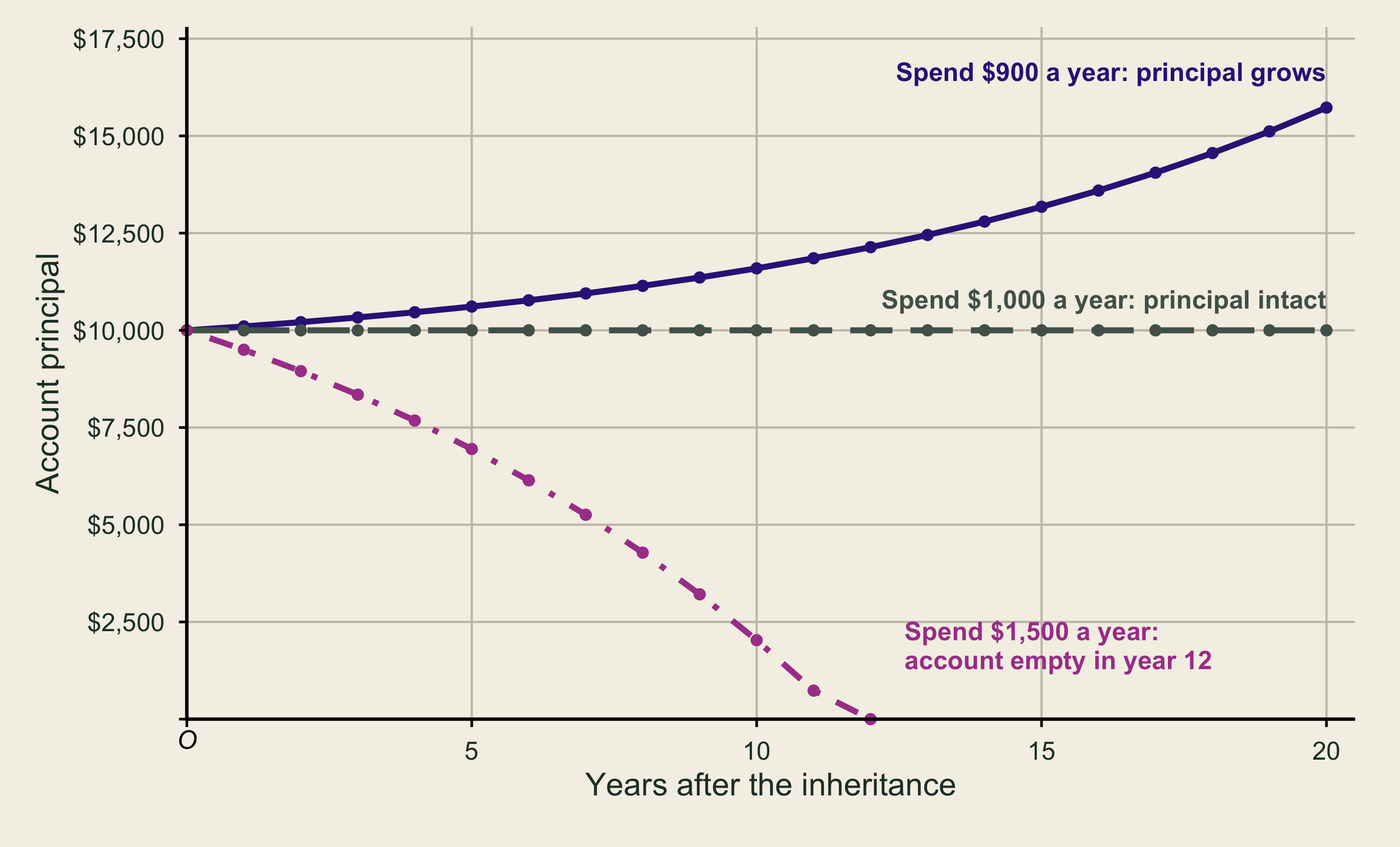
Spending $1,000 a year or less passes the sustainability test; spending more fails it. The Hartwick rule uses the same yardstick for an economy: watch the value of the principal. A principal that holds steady or grows signals a sustainable spending pattern, and a shrinking one signals an unsustainable pattern.

Natural capital, physical capital, and substitutability

The current generation inherits two kinds of capital: natural capital, the stock of environmental and natural resources, and physical capital, such as buildings, equipment, schools, and roads. Using this endowment sustainably means living off the services it provides while keeping its combined value, the principal, intact. Depleting a forest or an oil field is not the problem by itself. The problem is consuming its value without replacing it, so that later generations inherit less total capital.

Whether maintaining the combined value is enough depends on how easily physical capital can stand in for natural capital. If the substitution is easy, keeping the total value constant is sufficient. If it is not, investing in physical capital alone may not protect future well-being.

For some essential environmental resources, easy substitution is clearly unrealistic. Breathable air could in principle be replaced by air-conditioned domed cities, but the cost and artificiality would make that a poor form of compensation. Compensation across generations therefore has limits.

Example: Nauru

ImportantNauru: weak sustainability in the extreme

Limestone pinnacles left by phosphate mining on Nauru. Photo: Sean Kelleher, 2013, CC BY-SA 2.0, via Wikimedia Commons.

The weak sustainability criterion asks whether losses of natural capital are matched by enough new physical or financial capital to keep total capital from falling. Failing it signals unsustainable behavior; the harder question is whether passing it is enough.

Nauru is a small Pacific island about 3,000 kilometers northeast of Australia, with some of the highest-grade phosphate ever found. Phosphate is a key fertilizer ingredient. Mining ran for about a century, first under colonial powers and then, after independence, under Nauruans themselves. It made the remaining inhabitants richer, including through a trust fund once believed to hold over $1 billion, but it wiped out most of the island’s ecosystems. By the late 1990s, imports paid for with phosphate revenue met most local needs.

Whatever one thinks of Nauru’s choices, the strategy cannot work for the whole world: one country’s imports are another country’s exports. Meeting the weak criterion may be necessary for sustainability, but Nauru shows it is not always sufficient, which is why more demanding criteria are useful.

A postscript strengthens the lesson. The trust fund was later largely lost through poor investments and mismanagement, so even the financial capital meant to replace the phosphate was not maintained (Development Policy Centre).

Source: Tietenberg and Lewis (2023), Example 5.2, drawing on Gowdy and McDaniel (1999).

Weak, strong, and environmental sustainability

Because physical capital may not substitute well for natural capital, some economists propose stricter definitions of sustainability.

Definition	What must be maintained	Substitution assumption	Restrictiveness
Weak sustainability	The value of total capital, natural plus physical	Physical capital can substitute for natural capital	Less restrictive
Strong sustainability	The value of natural capital	Little or no substitution is possible	More restrictive
Environmental sustainability	The physical flows of key individual resources	Maintaining an aggregate value is not sufficient	Specific to each resource

Weak and strong sustainability both preserve an aggregate value rather than a specific physical flow. Strong sustainability assumes that natural capital drives future well-being, so it protects the value of natural capital itself. Environmental sustainability is more specific. For a fishery, it would require catch levels that do not exceed the growth of the fish population. For a wetland, it would require preserving specific ecological functions rather than merely their aggregate value.

19. Implications for environmental policy

Two criteria, four possible outcomes

Sustainability and efficiency are useful together only because they overlap partially. If they always agreed, one would be redundant; if they could never agree, policy would face an impossible choice. Some efficient allocations fail the sustainability test, some sustainable allocations waste net benefits, and some allocations pass both. Market outcomes can land in any of the four combinations.

	Efficient	Inefficient
Sustainable	Efficient and sustainable: the policy target	Sustainable, but net benefits are wasted
Unsustainable	Efficient, but later generations end up worse off	Inefficient and unsustainable: room for win–win reform

Sustainability as a constraint, efficiency as a guide

The partial overlap suggests a two-step strategy. First, treat sustainability as an overriding constraint: rule out allocations that leave later generations worse off. Second, among the allocations that remain, pick the one with the greatest dynamic or static efficiency, whichever fits the decision.

Each criterion does work the other cannot. By itself, the sustainability criterion cannot tell decision makers which of the infinite number of sustainable allocations to choose. Efficiency fills that gap by selecting the sustainable allocation that yields the greatest net benefit.

Win–win changes

The combination is especially useful because inefficiency is a common cause of unsustainable outcomes. Fixing the inefficiency can restore sustainability outright or bring the economy much closer to it.

Correcting inefficiencies can also produce win–win changes, in which every affected party can end up better off. Moving to an efficient allocation enlarges total net benefits, and part of that gain can compensate those who would otherwise lose, which weakens opposition to reform. By contrast, when a change costs the losers more than it gains the winners, no amount of compensation can leave everyone better off.

Whether markets and political institutions typically deliver allocations that pass both tests is a question for the chapters that follow.

20. Review of Sections 16–19

Key points for Sections 16–19

1. Efficiency is mainly concerned with eliminating waste. Intertemporal fairness asks what earlier generations owe later ones.
2. Rawls’s veil of ignorance motivates the sustainability criterion: future generations should be left no worse off than current generations.
3. In the neodymium model, the efficient allocation without sharing gives Period 2 $7,500, below the $8,593.75 each period would receive from an equal split. If Period 1 keeps $8,593.75 and invests the extra $781.25, Period 2 receives $9,062.50.
4. Efficient allocations do not automatically satisfy the sustainability criterion, but they can be compatible with it. In the neodymium example, compatibility requires that the sharing actually take place.
5. The Alaska Permanent Fund shares oil wealth across generations but falls short of full sustainability because it saves only part of the relevant royalty revenue (25% to 50%) and its principal could be spent by majority vote.
6. The Hartwick rule makes the criterion operational: invest all scarcity rent, and check each year whether the value of total capital is declining.
7. Nauru shows that weak sustainability may be necessary but is not always sufficient. Strong and environmental sustainability place greater weight on natural capital and on specific resource flows.
8. Good policy treats sustainability as a constraint and uses efficiency to choose among sustainable allocations. Correcting inefficiencies can create win–win changes.

Key terms for Sections 16–19

Term	Meaning here
Intertemporal fairness	Fair treatment of people living at different times, including future generations
Veil of ignorance	Rawls’s thought experiment in which people choose rules before knowing their position, or here their generation
Sustainability criterion	The standard that future generations should be left no worse off than current generations
Natural capital	Environmental and natural resources that provide a flow of services over time
Physical capital	Produced assets such as buildings, equipment, schools, and roads
Weak sustainability	Maintaining the value of total capital, natural plus physical
Strong sustainability	Maintaining the value of natural capital
Environmental sustainability	Maintaining the physical flows of key individual resources
Win–win change	A change after which every affected party can be made better off than before

Discussion questions for Sections 16–19

1. Alaska places 25% to 50% of certain mineral royalties in its Permanent Fund. What share of resource rent should a resource-rich state or country save for future residents? What political pressures push the share up or down?
2. Nauru may have satisfied the weak sustainability criterion while destroying most of its ecosystems. Which of the three definitions of sustainability would have flagged the problem, and why?
3. Environmental sustainability often requires maintaining a constant physical flow of individual resources, such as fish from the sea or wood from the forest, while weak and strong sustainability require maintaining an aggregate value. When might these criteria lead to different choices? Why? (Adapted from Tietenberg and Lewis 2023, Discussion Question 1, p. 127.)

References

• Alaska Permanent Fund Corporation. “Alaska Permanent Fund.” https://apfc.org. Accessed January 19, 2023, as reported in Tietenberg and Lewis (2023).
• Gowdy, John M., and Carl N. McDaniel. 1999. “The Physical Destruction of Nauru: An Example of Weak Sustainability.” Land Economics 75 (2): 333–338. https://doi.org/10.2307/3147015.
• Harris, Jonathan M., and Brian Roach. 2021. Environmental and Natural Resource Economics: A Contemporary Approach, 5th ed. “Resource Allocation Over Time,” pp. 119–135.
• Hartwick, John M. 1977. “Intergenerational Equity and the Investing of Rents from Exhaustible Resources.” American Economic Review 67 (5): 972–974. JSTOR.
• Rawls, John. 1971. A Theory of Justice. Cambridge, MA: Harvard University Press.
• Solow, Robert M. 1986. “On the Intergenerational Allocation of Natural Resources.” The Scandinavian Journal of Economics 88 (1): 141–149. https://doi.org/10.2307/3440280.
• Tietenberg, Tom, and Lynne Lewis. 2023. Environmental and Natural Resource Economics, 12th ed. New York: Routledge. “Dynamic Efficiency and Sustainable Development,” pp. 120–127. https://doi.org/10.4324/9781003213734.
• U.S. Department of Energy. 2022. Rare Earth Permanent Magnets: Supply Chain Deep Dive Assessment. Report.
• U.S. Geological Survey. 2026. “Rare Earths.” Mineral Commodity Summaries 2026. https://doi.org/10.3133/mcs2026.