Ducks Unlimited
On the $100 decision scale
- Cash you keep
- $75
- From your cash
- $5
- Donation support
- $5
- Total to organization
- $10
If selected: $7.50 cash to you. $0.50 from your cash + $0.50 support = $1 to Ducks Unlimited.
ECON 341 · Natural Resource Economics Instructor: Byeong-Hak Choe SUNY Geneseo · Fall 2026
Response data, regression interpretation, and supporting analysis
October 26, 2026
library(tidyverse)
forest_dir <- "../scripts/forest-choice"
source(file.path(forest_dir, "analysis.R"))
source(file.path(forest_dir, "model.R"))
source(file.path(forest_dir, "student-figures.R"))
source(file.path(forest_dir, "student-cards.R"))
# The private import script separates runs and retains one complete, valid
# submission per code before this page is rendered. No raw records are printed.
activity <- forest_load_responses(
params$responses_csv, file.path(forest_dir, "choice-design.csv"), params$run_id
)
responses <- activity$data |> as_tibble()
choices <- responses |>
filter(selected == 1) |>
select(participant_id, card_id, recipient, cost_dollars, cash_dollars,
donation_dollars, support_dollars, total_dollars)
people <- n_distinct(choices$participant_id)
choice_sets <- nrow(choices)
is_synthetic <- str_starts(activity$run_id, "SYNTHETIC-")
money <- function(x) sprintf("USD %.2f", x)
percent <- function(x) scales::percent(x, accuracy = 0.1)
donation_share <- mean(choices$recipient != "NONE")
matched_choices <- choices |> filter(card_id %in% sprintf("C%02d", 1:4))
import_summary <- if (!is_synthetic && file.exists(params$import_summary_csv))
read_csv(params$import_summary_csv, show_col_types = FALSE) else NULL
# Fit once. A valid set of choices is retained even if the model cannot be fit.
fit_error <- NULL
fit <- tryCatch(forest_fit_choice_model(responses), error = function(error) {
fit_error <<- conditionMessage(error)
NULL
})
coefficients <- if (!is.null(fit)) as_tibble(fit$coefficients) else
tibble(term = character(), estimate = double(), std_error = double(),
conf_low = double(), conf_high = double())
b_cost <- coefficients |> filter(term == "cost_dollars") |> pull(estimate)
b_gift <- coefficients |> filter(term == "donation_dollars") |> pull(estimate)
mwtp <- if (!is.null(fit)) as_tibble(fit$marginal_wtp) else
tibble(estimate = NA_real_, conf_low = NA_real_, conf_high = NA_real_,
status = "The regression could not be reliably estimated for this run.")
report_mwtp <- all(is.finite(c(mwtp$estimate, mwtp$conf_low, mwtp$conf_high)))
show_example <- report_mwtp && between(mwtp$estimate, 0, 1)Read the shorter student summary. This extended version includes the response-data structure, regression notation, log-relative-odds calculations, and the algebra behind the money trade-off.
Would you keep your cash, support Ducks Unlimited, or support Trout Unlimited? Open a card below to revisit the original offers. Everyone faced the same twelve menus; their order and the organizations’ left/right positions were shuffled. The labels C01–C12 identify the menus, rather than the order on your screen.
Large amounts are on the original display scale. Actual payments are 10%: giving up $5 on a card means giving up $0.50 in actual cash. Each option also shows its actual cash and donation.
Original offers · display amounts are paid at 10%
On the $100 decision scale
If selected: $7.50 cash to you. $0.50 from your cash + $0.50 support = $1 to Ducks Unlimited.
On the $100 decision scale
If selected: $7.50 cash to you. $0.50 from your cash + $0.50 support = $1 to Trout Unlimited.
On the $100 decision scale
If selected: $8 cash to you; no donation. The $2 support is unused.
Original offers · display amounts are paid at 10%
On the $100 decision scale
If selected: $6 cash to you. $2 from your cash + $2 support = $4 to Ducks Unlimited.
On the $100 decision scale
If selected: $6 cash to you. $2 from your cash + $2 support = $4 to Trout Unlimited.
On the $100 decision scale
If selected: $8 cash to you; no donation. The $2 support is unused.
Original offers · display amounts are paid at 10%
On the $100 decision scale
If selected: $5 cash to you. $3 from your cash + $1 support = $4 to Ducks Unlimited.
On the $100 decision scale
If selected: $5 cash to you. $3 from your cash + $1 support = $4 to Trout Unlimited.
On the $100 decision scale
If selected: $8 cash to you; no donation. The $2 support is unused.
Original offers · display amounts are paid at 10%
On the $100 decision scale
If selected: $0 cash to you. $8 from your cash + $2 support = $10 to Ducks Unlimited.
On the $100 decision scale
If selected: $0 cash to you. $8 from your cash + $2 support = $10 to Trout Unlimited.
On the $100 decision scale
If selected: $8 cash to you; no donation. The $2 support is unused.
Original offers · display amounts are paid at 10%
On the $100 decision scale
If selected: $7.50 cash to you. $0.50 from your cash + $0.50 support = $1 to Ducks Unlimited.
On the $100 decision scale
If selected: $7 cash to you. $1 from your cash + $0 support = $1 to Trout Unlimited.
On the $100 decision scale
If selected: $8 cash to you; no donation. The $2 support is unused.
Original offers · display amounts are paid at 10%
On the $100 decision scale
If selected: $7 cash to you. $1 from your cash + $0 support = $1 to Ducks Unlimited.
On the $100 decision scale
If selected: $7.50 cash to you. $0.50 from your cash + $0.50 support = $1 to Trout Unlimited.
On the $100 decision scale
If selected: $8 cash to you; no donation. The $2 support is unused.
Original offers · display amounts are paid at 10%
On the $100 decision scale
If selected: $6.50 cash to you. $1.50 from your cash + $0.50 support = $2 to Ducks Unlimited.
On the $100 decision scale
If selected: $6.50 cash to you. $1.50 from your cash + $1.50 support = $3 to Trout Unlimited.
On the $100 decision scale
If selected: $8 cash to you; no donation. The $2 support is unused.
Original offers · display amounts are paid at 10%
On the $100 decision scale
If selected: $6.50 cash to you. $1.50 from your cash + $1.50 support = $3 to Ducks Unlimited.
On the $100 decision scale
If selected: $6.50 cash to you. $1.50 from your cash + $0.50 support = $2 to Trout Unlimited.
On the $100 decision scale
If selected: $8 cash to you; no donation. The $2 support is unused.
Original offers · display amounts are paid at 10%
On the $100 decision scale
If selected: $5 cash to you. $3 from your cash + $2 support = $5 to Ducks Unlimited.
On the $100 decision scale
If selected: $3 cash to you. $5 from your cash + $0 support = $5 to Trout Unlimited.
On the $100 decision scale
If selected: $8 cash to you; no donation. The $2 support is unused.
Original offers · display amounts are paid at 10%
On the $100 decision scale
If selected: $3 cash to you. $5 from your cash + $0 support = $5 to Ducks Unlimited.
On the $100 decision scale
If selected: $5 cash to you. $3 from your cash + $2 support = $5 to Trout Unlimited.
On the $100 decision scale
If selected: $8 cash to you; no donation. The $2 support is unused.
Original offers · display amounts are paid at 10%
On the $100 decision scale
If selected: $4 cash to you. $4 from your cash + $0 support = $4 to Ducks Unlimited.
On the $100 decision scale
If selected: $4 cash to you. $4 from your cash + $2 support = $6 to Trout Unlimited.
On the $100 decision scale
If selected: $8 cash to you; no donation. The $2 support is unused.
Original offers · display amounts are paid at 10%
On the $100 decision scale
If selected: $4 cash to you. $4 from your cash + $2 support = $6 to Ducks Unlimited.
On the $100 decision scale
If selected: $4 cash to you. $4 from your cash + $0 support = $4 to Trout Unlimited.
On the $100 decision scale
If selected: $8 cash to you; no donation. The $2 support is unused.
Reopen the activity instructions.
Six menus use smaller costs (C01, C02, C05–C08); six use larger costs (C03, C04, C09–C12). Keeping all USD 8 is available every time.
| Cards | Held fixed | What changes? |
|---|---|---|
| C01–C04 | All financial amounts within each card | Organization |
| C05/C06 | USD 1 total gift | Personal cost: USD 0.50 or USD 1 |
| C07/C08 | USD 1.50 personal cost | Total gift: USD 2 or USD 3 |
| C09/C10 | USD 5 total gift | Personal cost: USD 3 or USD 5 |
| C11/C12 | USD 4 personal cost | Total gift: USD 4 or USD 6 |
Reversing the two organizations’ offers helps distinguish responses to money from preferences for a recipient. These are overlapping comparisons, rather than every possible cost/gift combination; cost and gift still tend to rise together.
Under the announced payment rule, one saved card is selected for each of two selected people. For each outcome, cash kept + total gift = USD 8 + support, at most USD 10. Two outcomes therefore cost at most USD 20. Support is already included in the total gift. The figures below describe choices; they do not record which payments or transfers were actually made.
cat(sprintf('<div class="fc-results-stats" aria-label="Summary of the analyzed choices">
<div class="fc-results-stat"><strong>%s</strong><span>participants</span></div>
<div class="fc-results-stat"><strong>%s</strong><span>recorded choices, twelve per person</span></div>
<div class="fc-results-stat"><strong>%s</strong><span>of choices directed a gift to conservation</span></div>
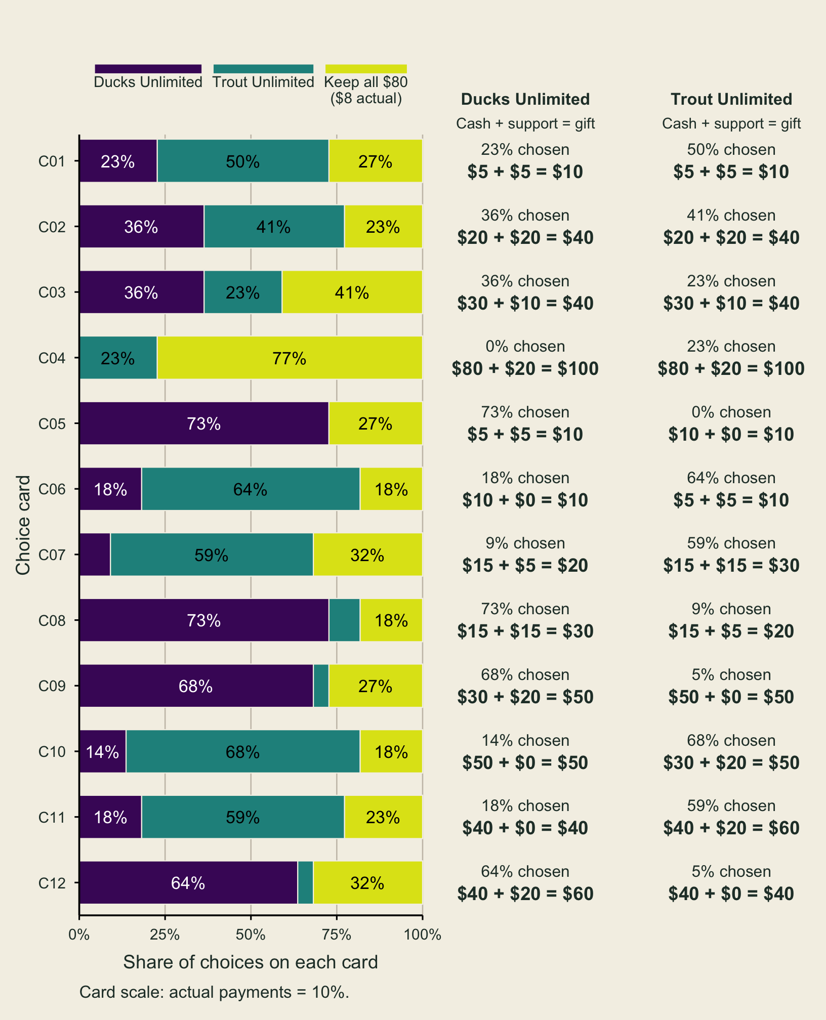
</div>', people, choice_sets, percent(donation_share)))These are the class’s recorded choices, summarized without names or individual response histories. Figure 1 uses the original card amounts so you can recognize the offers. The numerical summaries and regression use actual dollars. Expand Show R code to follow a calculation.
if (!is.null(import_summary)) {
audit <- import_summary[1, ]
cat(sprintf(paste0('::: {.callout-note title="Which submissions are included?"}\n\n',
'The export contained **%s completed class submissions** and **%s submissions ',
'from the earlier pilot run**. We analyze only the class run, with one complete, valid ',
'submission per code. '), audit$selected_run_submissions,
audit$other_run_submissions))
if (audit$repeat_submissions_removed == 0) {
cat('**The export contains one accepted submission per code within the class run.** ',
'Some codes appeared in both the earlier run and the class run; ',
'separating runs prevents those earlier choices from being counted again. ')
} else {
cat(sprintf(paste0('Where a code was submitted repeatedly within the class run, ',
'we kept its first complete, valid submission; **%s later submissions** ',
'were excluded under that rule. '), audit$repeat_submissions_removed))
}
cat('Codes identify records, so the file cannot establish whether one person ',
'used more than one code. Keeping cash and changing preferences between ',
'cards are valid choices, not grounds for exclusion.\n\n:::\n')
}The export contained 22 completed class submissions and 4 submissions from the earlier pilot run. We analyze only the class run, with one complete, valid submission per code. The export contains one accepted submission per code within the class run. Some codes appeared in both the earlier run and the class run; separating runs prevents those earlier choices from being counted again. Codes identify records, so the file cannot establish whether one person used more than one code. Keeping cash and changing preferences between cards are valid choices, not grounds for exclusion.
recipient_labels <- c(DU = "Ducks Unlimited", TU = "Trout Unlimited", NONE = "Keep cash")
recipient_summary <- choices |>
count(recipient, name = "choices") |>
complete(recipient = c("DU", "TU", "NONE"), fill = list(choices = 0)) |>
mutate(
recipient = recode(recipient, !!!recipient_labels),
share = percent(choices / sum(choices))
)
recipient_summary |>
knitr::kable(col.names = c("Option", "Times chosen", "Share of choices"))| Option | Times chosen | Share of choices |
|---|---|---|
| Ducks Unlimited | 95 | 36.0% |
| Keep cash | 80 | 30.3% |
| Trout Unlimited | 89 | 33.7% |
One person can choose different options on different cards. These are shares of 264 choices, rather than shares of different people.
Read across a row to see all three choices for the same card. Its shares use the same denominator: 22 participants. Keeping all $80 on the card ($8 actual cash) is shown alongside both donation options. The three shares add to 100% before rounding.
The bold offer amounts match the cards: from your cash + donation support = total gift. For example, $15 + $5 = $20 means an actual $1.50 contribution + $0.50 support = $2 donation. Cash kept on the card is $80 minus the displayed contribution; actual cash kept is 10% of that. Keeping all $80 means no contribution, no support used, and no donation.
The averages and regression below continue to use actual dollars.
These rows retain the original cards separately, even when one offer appears on more than one card. The competing offer can change, so the shares describe choices on the full menu. They do not isolate a causal effect of either cash contribution or donation support.
On C01–C04, the organizations had identical financial terms within each card. Those cards help compare recipients while holding the money amounts fixed.
On those 88 matched-card decisions, Ducks Unlimited received 23.9% of choices, Trout Unlimited 34.1%, and keeping cash 42.0%. Comparing these with the overall shares illustrates why financial terms matter. These descriptive differences do not establish a statistically clear preference between recipients.
choices |>
summarise(
`Personal cost` = mean(cost_dollars),
`Cash kept` = mean(cash_dollars),
`Support added` = mean(support_dollars),
`Total gift` = mean(donation_dollars)
) |>
pivot_longer(everything(), names_to = "Amount", values_to = "Mean") |>
mutate(Mean = money(Mean)) |>
knitr::kable(col.names = c("Amount", "Mean per recorded choice"))| Amount | Mean per recorded choice |
|---|---|
| Personal cost | USD 1.62 |
| Cash kept | USD 6.38 |
| Support added | USD 0.91 |
| Total gift | USD 2.53 |
These averages include keep-cash choices. Adding gifts across all twelve cards would overstate actual donations: only one saved card per selected person is implemented under the announced rule.
Every card has three offered alternatives. We retain all three rows for the regression, marking the chosen alternative with selected = 1. The other two rows tell the model what the person could have chosen.
For descriptive summaries, we filter to chosen rows. The analysis therefore uses 792 alternative rows, representing 264 decisions by 22 people. More rows do not create more independent participants.
The regression asks how recipient, personal cost, and total gift relate to choosing an option. It compares each donation option with keeping all cash, while accounting for the other offer on the same card.
The indices follow the structure of the response data:
participant_id.card_id. It is the card identifier, rather than the order in which it appeared on a screen.recipient values DU, TU, and NONE.Write p_{itj} for the probability that participant i chooses option j on card t, given all three offers on that card. Choosing j means selecting that offer; it is separate from the later payment draw. The probability p_{it0} refers to keeping all USD 8, our reference option.
For either donation option, the regression equation is:
\begin{aligned} &\log\left(\frac{p_{itj}}{p_{it0}}\right)\\ &\quad=\alpha_{DU}\,DU_{itj}+\alpha_{TU}\,TU_{itj}\\ &\qquad+\beta_g\,\text{Gift}_{itj}+\beta_c\,\text{Cost}_{itj}. \end{aligned}
| Regression term | Meaning |
|---|---|
| DU_{itj}, TU_{itj} | Recipient indicators: 1 for that organization and 0 otherwise |
| \text{Gift}_{itj} | Total actual dollars reaching the organization, including support |
| \text{Cost}_{itj} | Actual cash given up, relative to keeping USD 8 |
| p_{itj}/p_{it0} | How likely this participant is to choose this offer relative to keeping cash on this card |
For a given participant and card, the three probabilities—DU, TU, and keeping cash—sum to one. The coefficients are shared across participants and cards; the indices identify the observations to which the equation applies. The equation applies to each donation offer; the keep-cash reference has zero donation, zero personal cost, and both recipient indicators equal to zero.
One row is a participant–card–option combination (i,t,j). One decision is a participant–card combination (i,t), represented by three rows. The choice_set_id field groups those three rows. Each row records an available offer, and selected is 1 only for the offer actually chosen.
We can call that observed indicator y_{itj}: it is the row’s selected value, either 0 or 1. The probability p_{itj} is estimated by the regression; it is different from the observed indicator stored in the data frame.
The following rows are made-up illustrations, not an actual class response:
| Participant i | Card t | Option j | selected |
|---|---|---|---|
| Example participant | C07 | DU | 0 |
| Example participant | C07 | TU | 1 |
| Example participant | C07 | 0 (keep cash) | 0 |
The three rows describe one choice of TU, rather than three separate decisions. For every (i,t), the selected values sum to one. The model uses the two unchosen rows to learn what alternatives were available.
Each participant contributes 12\times3=36 rows. This run therefore has 22 participants × 12 cards × 3 options = 792 rows, representing 264 decisions. Repeated rows for one participant do not become additional independent participants; this is why uncertainty is clustered by participant.
The offer amounts happen to be the same across participants for a given card and organization. Keeping all three subscripts still makes each field’s connection to a data-frame row explicit.
There are two steps on the left side: form a probability ratio, then take its natural logarithm. Suppose, just for illustration, the probabilities are 40% DU, 20% TU, and 40% keeping cash. DU’s ratio relative to keeping cash is 0.40/0.40=1, and \log(1)=0.
| Probability ratio relative to keeping cash | Natural log of that ratio | Interpretation |
|---|---|---|
| 0.5 | About -0.693 | Half as likely as keeping cash |
| 1 | 0 | Equally likely as keeping cash |
| 2 | About 0.693 | Twice as likely as keeping cash |
A zero log ratio does not mean a zero probability. It means the offer and keeping cash have equal probabilities. A positive log ratio means the offer is more likely than keeping cash; a negative one means it is less likely.
Here, the ratio is p_{itj}/p_{it0}. Its denominator includes only keeping cash, rather than everyone who did not choose j. Students who select the other organization form a third group.
For the illustrative 40% DU / 20% TU / 40% cash probabilities, the ratio is 0.40/0.40=1. Dividing by 1-0.40=0.60 would instead compare DU with the other two choices combined. That is a different comparison from our equation.
A coefficient measures a change in the log probability ratio for a one-unit change in its variable. For cost and gift, one unit is one actual dollar. Taking the exponential converts the coefficient to a multiplier on the probability ratio:
\frac{\text{new ratio}}{\text{old ratio}} =\exp(\widehat\beta\,\Delta x).
if (!is.null(fit)) {
coefficients |>
filter(term %in% c("cost_dollars", "donation_dollars")) |>
mutate(
Variable = recode(term,
cost_dollars = "Personal cost: +USD 1, total gift fixed",
donation_dollars = "Total gift: +USD 1, personal cost fixed"),
Estimate = sprintf("%.3f", estimate),
`Odds factor` = sprintf("%.2f", exp(estimate)),
`95% CI` = sprintf("[%.3f, %.3f]", conf_low, conf_high)
) |>
select(Variable, Estimate, `Odds factor`, `95% CI`) |>
knitr::kable()
}| Variable | Estimate | Odds factor | 95% CI |
|---|---|---|---|
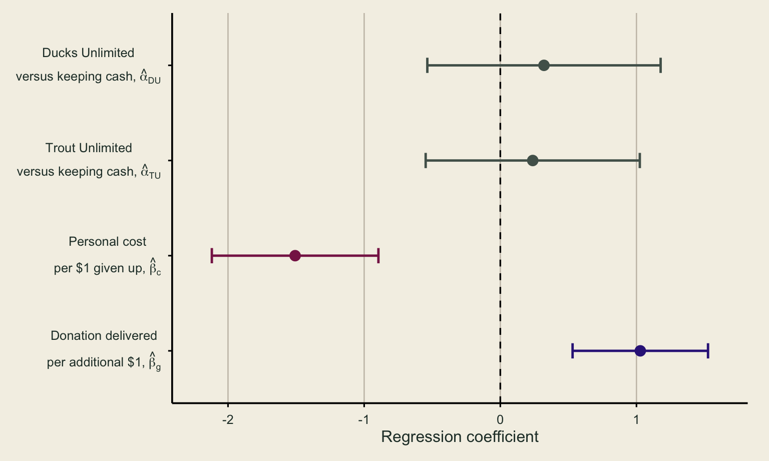
| Personal cost: +USD 1, total gift fixed | -1.507 | 0.22 | [-2.119, -0.895] |
| Total gift: +USD 1, personal cost fixed | 1.028 | 2.80 | [0.531, 1.526] |
Personal cost: an extra actual dollar multiplies the offer-to-cash probability ratio by 0.22, holding the total gift and recipient fixed. In this sample, that is about 77.8% lower relative odds. Total gift: an extra actual dollar reaching the same organization multiplies the ratio by 2.80, holding personal cost fixed.
Holding the total gift fixed while increasing personal cost means less instructor support. Holding personal cost fixed while increasing the gift means more support. These are the trade-offs built into the offers.
An odds multiplier is not a percentage-point change in probability. A multiplier of 2.80 means 2.80 times the previous offer-to-cash probability ratio. It does not mean an extra 2.80 percentage points, or a 280% probability. The new probabilities depend on all three options. Train (2009)
For a fixed participant i and card t, write r_{it,DU}=p_{it,DU}/p_{it0} and r_{it,TU}=p_{it,TU}/p_{it0}. Once the regression gives these two ratios, the three probabilities are:
\begin{aligned} p_{it0}&=\frac{1}{1+r_{it,DU}+r_{it,TU}},\\ p_{it,DU}&=\frac{r_{it,DU}}{1+r_{it,DU}+r_{it,TU}},\\ p_{it,TU}&=\frac{r_{it,TU}}{1+r_{it,DU}+r_{it,TU}}. \end{aligned}
The starting probabilities below are assumed teaching numbers, not fitted probabilities for an actual card. They give r_{it,DU}=1 and r_{it,TU}=0.5. Now increase only the DU gift by USD 1, with its personal cost unchanged; that requires USD 1 more support. A USD 4 gift at USD 4 personal cost, for example, could become a USD 5 gift with USD 1 support. The TU offer’s attributes stay fixed.
if (!is.null(fit)) {
new_ratios <- c(DU = exp(b_gift), TU = 0.5, cash = 1)
new_probabilities <- new_ratios / sum(new_ratios)
tibble(
Option = c("Ducks Unlimited", "Trout Unlimited", "Keep all USD 8"),
`Assumed starting probability` = percent(c(0.4, 0.2, 0.4)),
`After DU gift rises by USD 1` = percent(unname(new_probabilities))
) |>
knitr::kable()
} else {
knitr::asis_output("A numerical extension is not shown because no reliable gift coefficient is available for this run.")
}| Option | Assumed starting probability | After DU gift rises by USD 1 |
|---|---|---|
| Ducks Unlimited | 40.0% | 65.1% |
| Trout Unlimited | 20.0% | 11.6% |
| Keep all USD 8 | 40.0% | 23.3% |
Both the numerator and denominator matter. Even though the TU offer’s attributes have not changed, its probability can fall when DU becomes more attractive. Keeping the other offer fixed means fixing its financial terms and recipient, rather than fixing its choice probability.
People choose the option that provides the most utility, or well-being. We observe some attributes of that option, but not every influence on the person’s choice. A random utility model combines the observed attributes with an unobserved component, such as personal attachment to conservation.
Assumptions about that component let us estimate choice probabilities. “Random” refers to what the analyst does not observe; it does not mean people choose without preferences. This is separate from the winner-and-card draw. Train (2009, §2.3)
Repeated decisions: one person contributes twelve choices, so we use participant-clustered standard errors. The information comes from 22 people, not 264 independent people.
Confidence intervals: the dot is the sample estimate; its line shows uncertainty under the model and the approximate inference method. Crossing zero does not prove there is no relationship. The line also does not contain 95% of individual preferences. A small number of participants limits precision.
Recipient indicators: \widehat\alpha_{DU} and \widehat\alpha_{TU} compare a donation option with keeping cash at a zero-cost, zero-gift reference. Neither organization was offered with that financial profile. Their signs alone therefore do not tell us which organization people preferred at the actual offers.
The matched cards offer a direct recipient comparison at equal money amounts. Overlapping coefficient intervals do not, by themselves, test the difference between organizations.
The gift coefficient tells us how much an extra delivered dollar raises the fitted log relative odds. The cost coefficient tells us how much an extra dollar of personal cost lowers them. Their ratio asks: how much additional personal cash would just offset the attraction of one extra gift dollar?
\text{MWTP}=-\frac{\widehat\beta_g}{\widehat\beta_c}.
if (report_mwtp) {
cat(sprintf(paste0('::: {.callout-important title="Our estimated marginal trade-off"}\n\n',
'**%s of additional personal cash per additional USD 1 delivered** to the same organization. ',
'The approximate 95%% confidence interval is **%s to %s**.\n\n',
'For this sample, the fitted model predicts that these two changes offset ',
'each other when the recipient and the competing offer’s attributes stay fixed. ',
'This is a common marginal willingness to pay (MWTP) under the announced payment arrangement.\n\n:::\n'),
money(mwtp$estimate), money(mwtp$conf_low), money(mwtp$conf_high)))
} else {
cat('A reliable numerical MWTP is not reported for this run. ', mwtp$status,
' The ratio still explains the concept; a weak cost coefficient makes it unstable.')
}USD 0.68 of additional personal cash per additional USD 1 delivered to the same organization. The approximate 95% confidence interval is USD 0.60 to USD 0.76.
For this sample, the fitted model predicts that these two changes offset each other when the recipient and the competing offer’s attributes stay fixed. This is a common marginal willingness to pay (MWTP) under the announced payment arrangement.
This concerns an increase from a starting offer. The extra delivered dollar is added to the gift already being considered; the extra personal cost is added to that offer’s existing cost. The ratio does not tell us that the original gift is worth only this amount, or that everyone has the same maximum donation.
Start with an offered option that costs USD 4, leaves USD 4 cash, and delivers USD 4 without support. Raise the gift to USD 5. The fitted trade-off adds MWTP to personal cost, and instructor support funds the rest of the additional gift dollar:
if (show_example) {
tibble(
Scenario = c("Starting offer", "Regression prediction"),
personal_cost = c(4, 4 + mwtp$estimate),
total_gift = c(4, 5)
) |>
mutate(cash_kept = 8 - personal_cost,
support = total_gift - personal_cost) |>
select(Scenario, personal_cost, cash_kept, support, total_gift) |>
mutate(across(where(is.numeric), money)) |>
knitr::kable(col.names = c("Scenario", "Personal cost", "Cash kept", "Support", "Total gift"))
} else {
knitr::asis_output("No numerical interpolation is shown: MWTP is either too uncertain to report or would require a cost/support combination outside this local comparison.")
}| Scenario | Personal cost | Cash kept | Support | Total gift |
|---|---|---|---|---|
| Starting offer | USD 4.00 | USD 4.00 | USD 0.00 | USD 4.00 |
| Regression prediction | USD 4.68 | USD 3.32 | USD 0.32 | USD 5.00 |
In the prediction, you give up an additional USD 0.68, so the cash kept falls from USD 4 to USD 3.32. The organization receives USD 1 more. Support rises by USD 0.32, because the additional gift must equal the additional personal contribution plus the additional support.
The two offers have the same fitted log relative odds. With the competing offer and keep-cash option unchanged, the model also gives the same three choice probabilities. This does not mean every participant would personally be indifferent; the calculation uses common estimated coefficients.
The second row is an interpolated prediction, rather than an offered card or a payment. Its personal cost lies between observed USD 4 and USD 5 costs, and its support lies between USD 0 and USD 1. We show it only when the estimated trade-off keeps both amounts inside this feasible local comparison.
Holding the recipient fixed, the change in the fitted log ratio is:
\begin{aligned} &\Delta\log\left(\frac{p_{itj}}{p_{it0}}\right)\\ &\quad=\widehat\beta_g\,\Delta\text{Gift}_{itj} +\widehat\beta_c\,\Delta\text{Cost}_{itj}. \end{aligned}
For an unchanged ratio, set this expression equal to zero. Setting the gift increase to one dollar then gives \Delta\text{Cost}_{itj}=-\widehat\beta_g/\widehat\beta_c.
Using the unrounded estimates, 1.028 × 1 + (-1.507) × 0.682 is approximately zero. The positive gift effect and negative cost effect offset. Exponentiating that zero change gives an odds multiplier of one.
With a positive gift coefficient and a negative cost coefficient:
| Extra cost for the same extra USD 1 gift | Predicted effect on the offer-to-cash ratio |
|---|---|
| Less than MWTP | The offer becomes more attractive: the ratio rises |
| Exactly MWTP | The two effects offset: the ratio is unchanged |
| More than MWTP | The offer becomes less attractive: the ratio falls |
These comparisons hold the recipient and competing offer’s attributes fixed. Feasibility also requires sufficient support and enough personal cash.
WTP asks about a specified change: what is the most personal cash someone would give up for that change, relative to a stated starting point? An example would be a defined improvement to a park.
MWTP asks about one extra unit: here, the unit is an additional dollar reaching the same conservation organization. Our ratio describes the additional cash cost that offsets that extra delivered dollar under the model.
The estimate is not a percentage of students or a change in choice probability. It is measured in actual cash dollars per additional gift dollar. It also does not locate each person’s exact maximum WTP.
This is not total WTP for nature or for either organization. Multiplying the ratio by an entire gift ignores the starting point, recipient effects, and observed range. Extending this small-stakes estimate to a large park project would also assume the same trade-off holds far beyond the offers.
The interval combines the uncertainty and covariance of both financial coefficients, using a delta-method approximation. It concerns the estimated common trade-off, rather than the range containing 95% of students’ MWTP.
if (report_mwtp) {
cat(case_when(
mwtp$conf_low <= 1 && mwtp$conf_high >= 1 ~
"The interval includes USD 1, so it does not clearly distinguish the common trade-off from one dollar of personal cash per additional dollar delivered.",
mwtp$conf_high < 1 ~
"The entire approximate interval is below USD 1 of personal cash per additional dollar delivered.",
TRUE ~ "The entire approximate interval is above USD 1 of personal cash per additional dollar delivered."
))
}The entire approximate interval is below USD 1 of personal cash per additional dollar delivered.
If the personal-cost coefficient is near zero or has the wrong sign, the ratio becomes unstable. A numerical estimate or its interval may then be withheld, while all valid choices remain in the descriptive results. With only 22 participant clusters, the reported uncertainty is approximate.
| What the evidence can address | What it does not establish |
|---|---|
| Responses to personal cost and delivered funding | Each person’s exact maximum WTP |
| Recipient preferences at the offered financial terms | The total value of nature |
| A common marginal cash/gift trade-off under this arrangement | WTP for a guaranteed number of acres, species, or restored stream miles |
The gifts are unrestricted contributions. Choices can reflect trust in an organization, satisfaction from giving, provided cash, and available donation support, as well as concern for conservation. Hungerman and Ottoni-Wilhelm (2021) The same person may value a specified environmental improvement differently when it is funded through another mechanism. Kotchen (2015)
1. Why might a larger gift attract more choices when personal cost stays fixed?
The participant keeps the same amount of cash, while more money reaches conservation. Someone who values the organization’s work may therefore find the offer more attractive. In these cards, the larger gift at the same personal cost comes from additional instructor support.
In the regression, a positive \widehat\beta_g means an extra delivered dollar raises the offer-to-cash probability ratio, holding the recipient and personal cost fixed. It need not change everyone’s choice: people differ in their preferences, and the competing organization remains available. The gift supports the organization’s work but does not guarantee a specified number of acres or species protected.
2. On a matched card, what could explain preferring one recipient?
On a matched card, personal cost, cash kept, support, and total gift are the same for both organizations. A difference in choices can therefore reflect preferences for their causes, confidence in how they use donations, familiarity, past experience, or attachment to the places and wildlife they support.
Someone may prefer stream and fish habitat because they visit rivers. Another may care about protecting wetlands or wildlife they never expect to see, expressing existence or bequest value. The activity measures choices between the organization-and-cause bundles; it does not separately identify every reason behind them. A raw difference in this small sample also does not, by itself, establish a precise population-wide recipient preference.
3. Why can a donation trade-off differ from WTP for a specific park improvement?
A donation delivers money to an organization, which decides how to use it. A park-improvement valuation instead specifies a change, such as a safer trail or restored habitat, relative to a defined starting point. These are different objects of choice. A person may trust an organization, enjoy the act of contributing, or care about its broader mission without placing the same value on every project it could fund.
The payment setting matters too. Here, participants choose with provided cash, donation support, and a chance that one decision will be implemented. A park fee or tax may involve earned income, different access benefits, and a different connection between payment and environmental outcomes. Both use value and non-use value may matter, but their mix can change.
Our MWTP is a marginal cash-per-extra-gift-dollar trade-off under this arrangement. It cannot be multiplied by a proposed park budget to recover total park value, or treated as each person’s maximum payment for a defined improvement.
Train, Kenneth E. 2009. Discrete Choice Methods with Simulation, 2nd ed. Cambridge University Press.
Hungerman, Daniel M., and Mark Ottoni-Wilhelm. 2021. “Impure Impact Giving: Theory and Evidence.” Journal of Political Economy 129 (5): 1553–1614.
Kotchen, Matthew J. 2015. “Reconsidering Donations for Nonmarket Valuation.” Environmental and Resource Economics 62: 481–490.
---
title: "Classwork 6: Forest Choice Results — Extended"
subtitle: "Response data, regression interpretation, and supporting analysis"
date: 2026-10-26
filters:
- ../filters/course-tab-title.lua
title-prefix: ""
title-block-banner: false
toc: true
toc-depth: 3
toc-expand: 1
css:
- ../assets/css/econ-341-forest-choice.css
- ../assets/css/econ-341-forest-choice-results.css
format:
html:
code-fold: true
code-summary: "Show R code"
code-tools: true
html-math-method: katex
link-external-newwindow: true
execute:
eval: true
echo: true
warning: false
message: false
params:
responses_csv: "../scripts/forest-choice/data/2026-10-26/Responses-class-clean.csv"
run_id: "CONSERVATION-CLASS-01"
import_summary_csv: "../scripts/forest-choice/data/2026-10-26/import-summary.csv"
---
```{r}
#| label: prepare-results
library(tidyverse)
forest_dir <- "../scripts/forest-choice"
source(file.path(forest_dir, "analysis.R"))
source(file.path(forest_dir, "model.R"))
source(file.path(forest_dir, "student-figures.R"))
source(file.path(forest_dir, "student-cards.R"))
# The private import script separates runs and retains one complete, valid
# submission per code before this page is rendered. No raw records are printed.
activity <- forest_load_responses(
params$responses_csv, file.path(forest_dir, "choice-design.csv"), params$run_id
)
responses <- activity$data |> as_tibble()
choices <- responses |>
filter(selected == 1) |>
select(participant_id, card_id, recipient, cost_dollars, cash_dollars,
donation_dollars, support_dollars, total_dollars)
people <- n_distinct(choices$participant_id)
choice_sets <- nrow(choices)
is_synthetic <- str_starts(activity$run_id, "SYNTHETIC-")
money <- function(x) sprintf("USD %.2f", x)
percent <- function(x) scales::percent(x, accuracy = 0.1)
donation_share <- mean(choices$recipient != "NONE")
matched_choices <- choices |> filter(card_id %in% sprintf("C%02d", 1:4))
import_summary <- if (!is_synthetic && file.exists(params$import_summary_csv))
read_csv(params$import_summary_csv, show_col_types = FALSE) else NULL
# Fit once. A valid set of choices is retained even if the model cannot be fit.
fit_error <- NULL
fit <- tryCatch(forest_fit_choice_model(responses), error = function(error) {
fit_error <<- conditionMessage(error)
NULL
})
coefficients <- if (!is.null(fit)) as_tibble(fit$coefficients) else
tibble(term = character(), estimate = double(), std_error = double(),
conf_low = double(), conf_high = double())
b_cost <- coefficients |> filter(term == "cost_dollars") |> pull(estimate)
b_gift <- coefficients |> filter(term == "donation_dollars") |> pull(estimate)
mwtp <- if (!is.null(fit)) as_tibble(fit$marginal_wtp) else
tibble(estimate = NA_real_, conf_low = NA_real_, conf_high = NA_real_,
status = "The regression could not be reliably estimated for this run.")
report_mwtp <- all(is.finite(c(mwtp$estimate, mwtp$conf_low, mwtp$conf_high)))
show_example <- report_mwtp && between(mwtp$estimate, 0, 1)
```
[Read the shorter student summary](../econ-cw/econ-341-cw-06.html).
This extended version includes the response-data structure, regression notation,
log-relative-odds calculations, and the algebra behind the money trade-off.
## 1. Revisit the twelve choices
**Would you keep your cash, support Ducks Unlimited, or support Trout Unlimited?**
Open a card below to revisit the original offers. Everyone faced the same twelve
menus; their order and the organizations’ left/right positions were shuffled.
The labels C01–C12 identify the menus, rather than the order on your screen.
**Large amounts are on the original display scale. Actual payments are 10%:**
giving up $5 on a card means giving up $0.50 in actual cash. Each option also
shows its actual cash and donation.
```{r}
#| label: original-choice-cards
# Illustrate all three options directly from the validated design, without
# submitting anything or displaying anyone's recorded choices.
forest_student_card_gallery(activity$design)
```
[Reopen the activity instructions](../econ-cw-q/econ-341-cw-06-experiment.html).
::: {.callout-note title="What changes across cards?"}
- **Recipient:** wetlands and waterfowl habitat through Ducks Unlimited, or
rivers, streams, and coldwater fisheries through Trout Unlimited.
- **Personal cost:** the actual cash you give up, from USD 0.50 to USD 8.
- **Total gift:** the actual amount the organization receives, including support.
Six menus use smaller costs (C01, C02, C05–C08); six use larger costs
(C03, C04, C09–C12). **Keeping all USD 8 is available every time.**
:::
::: {.fc-results-detail}
<details>
<summary>How the comparisons separate cost, gift size, and recipient</summary>
| Cards | Held fixed | What changes? |
|:--|:--|:--|
| C01–C04 | All financial amounts within each card | Organization |
| C05/C06 | USD 1 total gift | Personal cost: USD 0.50 or USD 1 |
| C07/C08 | USD 1.50 personal cost | Total gift: USD 2 or USD 3 |
| C09/C10 | USD 5 total gift | Personal cost: USD 3 or USD 5 |
| C11/C12 | USD 4 personal cost | Total gift: USD 4 or USD 6 |
Reversing the two organizations’ offers helps distinguish responses to money
from preferences for a recipient. These are overlapping comparisons, rather
than every possible cost/gift combination; cost and gift still tend to rise
together.
Under the announced payment rule, one saved card is selected for each of two
selected people. For each outcome, **cash kept + total gift = USD 8 + support**,
at most USD 10. Two outcomes therefore cost at most USD 20. Support is already
included in the total gift. The figures below describe choices; they do not
record which payments or transfers were actually made.
</details>
:::
## 2. Our results at a glance
```{r}
#| label: results-at-a-glance
#| results: asis
cat(sprintf('<div class="fc-results-stats" aria-label="Summary of the analyzed choices">
<div class="fc-results-stat"><strong>%s</strong><span>participants</span></div>
<div class="fc-results-stat"><strong>%s</strong><span>recorded choices, twelve per person</span></div>
<div class="fc-results-stat"><strong>%s</strong><span>of choices directed a gift to conservation</span></div>
</div>', people, choice_sets, percent(donation_share)))
```
`r if (is_synthetic) "**Practice data:** these choices were simulated, rather than collected from the class." else "These are the class’s recorded choices, summarized without names or individual response histories."`
Figure 1 uses the **original card amounts** so you can recognize the offers.
The numerical summaries and regression use **actual dollars**. Expand
**Show R code** to follow a calculation.
```{r}
#| label: explain-data-cleaning
#| results: asis
if (!is.null(import_summary)) {
audit <- import_summary[1, ]
cat(sprintf(paste0('::: {.callout-note title="Which submissions are included?"}\n\n',
'The export contained **%s completed class submissions** and **%s submissions ',
'from the earlier pilot run**. We analyze only the class run, with one complete, valid ',
'submission per code. '), audit$selected_run_submissions,
audit$other_run_submissions))
if (audit$repeat_submissions_removed == 0) {
cat('**The export contains one accepted submission per code within the class run.** ',
'Some codes appeared in both the earlier run and the class run; ',
'separating runs prevents those earlier choices from being counted again. ')
} else {
cat(sprintf(paste0('Where a code was submitted repeatedly within the class run, ',
'we kept its first complete, valid submission; **%s later submissions** ',
'were excluded under that rule. '), audit$repeat_submissions_removed))
}
cat('Codes identify records, so the file cannot establish whether one person ',
'used more than one code. Keeping cash and changing preferences between ',
'cards are valid choices, not grounds for exclusion.\n\n:::\n')
}
```
### Which option was chosen most often?
```{r}
#| label: recipient-choice-summary
recipient_labels <- c(DU = "Ducks Unlimited", TU = "Trout Unlimited", NONE = "Keep cash")
recipient_summary <- choices |>
count(recipient, name = "choices") |>
complete(recipient = c("DU", "TU", "NONE"), fill = list(choices = 0)) |>
mutate(
recipient = recode(recipient, !!!recipient_labels),
share = percent(choices / sum(choices))
)
recipient_summary |>
knitr::kable(col.names = c("Option", "Times chosen", "Share of choices"))
```
One person can choose different options on different cards. These are shares
of **`r choice_sets` choices**, rather than shares of different people.
```{r}
#| label: fig-forest-results-shares
#| fig-width: 8.5
#| fig-height: 10.5
#| fig-cap: "All three choice shares on each card. Financial amounts use the original card scale: actual payments are 10% of those amounts. Keeping $80 on the card means keeping $8 actual cash. The offer columns show cash contribution + donation support = total gift. Viridis colors identify the three choices; each bar sums to 100% before rounding."
#| fig-alt: "Twelve horizontal stacked bars show all three choice shares for cards C01 to C12. Large bold financial labels use the original card amounts for Ducks Unlimited and Trout Unlimited. They show cash contribution plus donation support equals total gift. The keep-all-80-dollars option corresponds to eight dollars of actual cash, and every displayed financial amount is paid at ten percent."
card_shares <- responses |>
group_by(card_id, recipient, cost_dollars, support_dollars, donation_dollars) |>
summarise(shown = n(), chosen = sum(selected), .groups = "drop") |>
mutate(share = chosen / shown)
forest_student_card_plot(card_shares)
```
[Enlarge Figure 1](econ-341-cw-06-extended_files/figure-html/fig-forest-results-shares-1.png){target="_blank" rel="noopener noreferrer"}
**Read across a row to see all three choices for the same card.** Its shares
use the same denominator: **`r people` participants**. Keeping all **$80 on
the card ($8 actual cash)** is shown alongside both donation options. The three shares add to
100% before rounding.
The bold offer amounts match the cards: **from your cash + donation support =
total gift**. For example, **$15 + $5 = $20** means an actual **$1.50
contribution + $0.50 support = $2 donation**. Cash kept on the card is
**$80 minus the displayed contribution**; actual cash kept is 10% of that.
Keeping all $80 means no contribution, no support used, and no donation.
**The averages and regression below continue to use actual dollars.**
These rows retain the original cards separately, even when one offer appears
on more than one card. The competing offer can change, so the shares describe
choices on the full menu. They do not isolate a causal effect of either cash
contribution or donation support.
On C01–C04, the organizations had identical financial terms within each card.
Those cards help compare recipients while holding the money amounts fixed.
On those **`r nrow(matched_choices)` matched-card decisions**, Ducks Unlimited
received **`r percent(mean(matched_choices$recipient == "DU"))`** of choices,
Trout Unlimited **`r percent(mean(matched_choices$recipient == "TU"))`**, and
keeping cash **`r percent(mean(matched_choices$recipient == "NONE"))`**.
Comparing these with the overall shares illustrates why financial terms
matter. These descriptive differences do not establish a statistically clear
preference between recipients.
### How much cash and conservation funding did people choose?
```{r}
#| label: average-allocations
choices |>
summarise(
`Personal cost` = mean(cost_dollars),
`Cash kept` = mean(cash_dollars),
`Support added` = mean(support_dollars),
`Total gift` = mean(donation_dollars)
) |>
pivot_longer(everything(), names_to = "Amount", values_to = "Mean") |>
mutate(Mean = money(Mean)) |>
knitr::kable(col.names = c("Amount", "Mean per recorded choice"))
```
These averages include keep-cash choices. **Adding gifts across all twelve
cards would overstate actual donations:** only one saved card per selected
person is implemented under the announced rule.
::: {.fc-results-detail}
<details>
<summary>Why the data have three rows per decision</summary>
Every card has three offered alternatives. We retain all three rows for the
regression, marking the chosen alternative with `selected = 1`. The other
two rows tell the model what the person could have chosen.
For descriptive summaries, we filter to chosen rows. The analysis therefore
uses **`r nrow(responses)` alternative rows**, representing
**`r choice_sets` decisions by `r people` people**. More rows do not create
more independent participants.
</details>
:::
## 3. What does the regression tell us?
The regression asks how **recipient, personal cost, and total gift** relate
to choosing an option. It compares each donation option with keeping all cash,
while accounting for the other offer on the same card.
The indices follow the structure of the response data:
- **$i$ identifies the participant.** In the prepared data frame, this is
`participant_id`.
- **$t$ identifies the card**, such as C01 or C07, using `card_id`. It is the
card identifier, rather than the order in which it appeared on a screen.
- **$j$ identifies an option on that card:** DU, TU, or $0$ for keeping cash.
These correspond to `recipient` values `DU`, `TU`, and `NONE`.
Write $p_{itj}$ for the probability that **participant $i$ chooses option $j$
on card $t$**, given all three offers on that card. Choosing $j$ means selecting
that offer; it is separate from the later payment draw. The probability
$p_{it0}$ refers to keeping all USD 8, our **reference option**.
For either donation option, the regression equation is:
$$
\begin{aligned}
&\log\left(\frac{p_{itj}}{p_{it0}}\right)\\
&\quad=\alpha_{DU}\,DU_{itj}+\alpha_{TU}\,TU_{itj}\\
&\qquad+\beta_g\,\text{Gift}_{itj}+\beta_c\,\text{Cost}_{itj}.
\end{aligned}
$$
| Regression term | Meaning |
|:--|:--|
| $DU_{itj}$, $TU_{itj}$ | Recipient indicators: 1 for that organization and 0 otherwise |
| $\text{Gift}_{itj}$ | Total actual dollars reaching the organization, including support |
| $\text{Cost}_{itj}$ | Actual cash given up, relative to keeping USD 8 |
| $p_{itj}/p_{it0}$ | How likely this participant is to choose this offer relative to keeping cash on this card |
For a given participant and card, the three probabilities—DU, TU, and keeping
cash—sum to one. The coefficients are shared across participants and cards;
the indices identify the observations to which the equation applies.
The equation applies to each donation offer; the keep-cash reference has
zero donation, zero personal cost, and both recipient indicators equal to zero.
### How the indices correspond to data-frame rows
**One row is a participant–card–option combination $(i,t,j)$. One decision is
a participant–card combination $(i,t)$, represented by three rows.** The
`choice_set_id` field groups those three rows. Each row records an available
offer, and `selected` is 1 only for the offer actually chosen.
We can call that observed indicator $y_{itj}$: it is the row’s `selected`
value, either 0 or 1. The probability $p_{itj}$ is estimated by the regression;
it is different from the observed indicator stored in the data frame.
The following rows are **made-up illustrations**, not an actual class response:
| Participant $i$ | Card $t$ | Option $j$ | `selected` |
|:--|:--|:--|--:|
| Example participant | C07 | DU | 0 |
| Example participant | C07 | TU | 1 |
| Example participant | C07 | $0$ (keep cash) | 0 |
The three rows describe **one choice of TU**, rather than three separate
decisions. For every $(i,t)$, the `selected` values sum to one. The model
uses the two unchosen rows to learn what alternatives were available.
Each participant contributes $12\times3=36$ rows. This run therefore has
**`r people` participants × 12 cards × 3 options = `r nrow(responses)` rows**,
representing **`r choice_sets` decisions**. Repeated rows for one participant
do not become additional independent participants; this is why uncertainty
is clustered by participant.
The offer amounts happen to be the same across participants for a given
card and organization. Keeping all three subscripts still makes each
field’s connection to a data-frame row explicit.
### Understanding log relative odds
There are two steps on the left side: **form a probability ratio, then take
its natural logarithm**. Suppose, just for illustration, the probabilities
are 40% DU, 20% TU, and 40% keeping cash. DU’s ratio relative to keeping cash
is $0.40/0.40=1$, and $\log(1)=0$.
| Probability ratio relative to keeping cash | Natural log of that ratio | Interpretation |
|:--|:--|:--|
| $0.5$ | About $-0.693$ | Half as likely as keeping cash |
| $1$ | $0$ | Equally likely as keeping cash |
| $2$ | About $0.693$ | Twice as likely as keeping cash |
**A zero log ratio does not mean a zero probability.** It means the offer
and keeping cash have equal probabilities. A positive log ratio means the
offer is more likely than keeping cash; a negative one means it is less likely.
::: {.callout-note title="The denominator matters with three choices"}
Here, the ratio is $p_{itj}/p_{it0}$. Its denominator includes
**only keeping cash**, rather than everyone who did not choose $j$.
Students who select the other organization form a third group.
For the illustrative 40% DU / 20% TU / 40% cash probabilities, the ratio
is $0.40/0.40=1$. Dividing by $1-0.40=0.60$ would instead compare DU with
the other two choices combined. That is a different comparison from our equation.
:::
### Coefficients and their uncertainty
```{r}
#| label: fig-forest-results-coefficients
#| fig-width: 8
#| fig-height: 4.8
#| fig-cap: "Dots are regression estimates; lines are approximate 95% confidence intervals using participant-clustered standard errors. Each label gives the verbal meaning followed by the coefficient notation. Personal cost is red, total gift is blue, and recipient indicators are neutral. Monetary effects use actual dollars."
#| fig-alt: "Regression coefficient estimates with horizontal 95 percent confidence intervals and a dashed zero reference line. Labels identify Ducks Unlimited with alpha DU, Trout Unlimited with alpha TU, personal cost with beta c, and total gift with beta g."
if (!is.null(fit)) {
coefficients |>
select(term, estimate, std_error, conf_low, conf_high) |>
forest_student_coefficient_plot()
} else {
knitr::asis_output(paste("The regression could not be reliably estimated:",
fit_error, "The descriptive results retain every valid choice."))
}
```
A coefficient measures a change in the **log probability ratio** for a
one-unit change in its variable. For cost and gift, one unit is **one actual
dollar**. Taking the exponential converts the coefficient to a multiplier
on the probability ratio:
$$
\frac{\text{new ratio}}{\text{old ratio}}
=\exp(\widehat\beta\,\Delta x).
$$
```{r}
#| label: interpret-financial-coefficients
if (!is.null(fit)) {
coefficients |>
filter(term %in% c("cost_dollars", "donation_dollars")) |>
mutate(
Variable = recode(term,
cost_dollars = "Personal cost: +USD 1, total gift fixed",
donation_dollars = "Total gift: +USD 1, personal cost fixed"),
Estimate = sprintf("%.3f", estimate),
`Odds factor` = sprintf("%.2f", exp(estimate)),
`95% CI` = sprintf("[%.3f, %.3f]", conf_low, conf_high)
) |>
select(Variable, Estimate, `Odds factor`, `95% CI`) |>
knitr::kable()
}
```
`r if (!is.null(fit)) sprintf("**Personal cost:** an extra actual dollar multiplies the offer-to-cash probability ratio by %.2f, holding the total gift and recipient fixed. In this sample, that is about %.1f%% lower relative odds. **Total gift:** an extra actual dollar reaching the same organization multiplies the ratio by %.2f, holding personal cost fixed.", exp(b_cost), 100 * (1 - exp(b_cost)), exp(b_gift)) else "The table is unavailable because this run does not support a reliable regression fit. The interpretation of a coefficient as a change in log relative odds still applies to the model."`
Holding the total gift fixed while increasing personal cost means less
instructor support. Holding personal cost fixed while increasing the gift
means more support. These are the trade-offs built into the offers.
**An odds multiplier is not a percentage-point change in probability.** A
multiplier of 2.80 means 2.80 times the previous offer-to-cash probability
ratio. It does not mean an extra 2.80 percentage points, or a 280% probability.
The new probabilities depend on all three options.
[Train (2009)](https://eml.berkeley.edu/books/choice2.html){target="_blank" rel="noopener noreferrer"}
::: {.fc-results-detail}
<details>
<summary>Worked example: converting relative odds back into three probabilities</summary>
For a fixed participant $i$ and card $t$, write
$r_{it,DU}=p_{it,DU}/p_{it0}$ and
$r_{it,TU}=p_{it,TU}/p_{it0}$. Once the regression gives these two ratios,
the three probabilities are:
$$
\begin{aligned}
p_{it0}&=\frac{1}{1+r_{it,DU}+r_{it,TU}},\\
p_{it,DU}&=\frac{r_{it,DU}}{1+r_{it,DU}+r_{it,TU}},\\
p_{it,TU}&=\frac{r_{it,TU}}{1+r_{it,DU}+r_{it,TU}}.
\end{aligned}
$$
The starting probabilities below are **assumed teaching numbers**, not fitted
probabilities for an actual card. They give $r_{it,DU}=1$ and $r_{it,TU}=0.5$.
Now increase only the DU gift by USD 1, with its personal cost unchanged;
that requires USD 1 more support. A USD 4 gift at USD 4 personal cost, for
example, could become a USD 5 gift with USD 1 support. The TU offer’s
attributes stay fixed.
```{r}
#| label: log-odds-probability-example
if (!is.null(fit)) {
new_ratios <- c(DU = exp(b_gift), TU = 0.5, cash = 1)
new_probabilities <- new_ratios / sum(new_ratios)
tibble(
Option = c("Ducks Unlimited", "Trout Unlimited", "Keep all USD 8"),
`Assumed starting probability` = percent(c(0.4, 0.2, 0.4)),
`After DU gift rises by USD 1` = percent(unname(new_probabilities))
) |>
knitr::kable()
} else {
knitr::asis_output("A numerical extension is not shown because no reliable gift coefficient is available for this run.")
}
```
Both the numerator and denominator matter. Even though the TU offer’s
attributes have not changed, its **probability** can fall when DU becomes
more attractive. Keeping the other offer fixed means fixing its financial
terms and recipient, rather than fixing its choice probability.
</details>
:::
::: {.callout-note title="The idea behind a random utility model (RUM)" collapse="true"}
People choose the option that provides the most utility, or well-being.
We observe some attributes of that option, but not every influence on the
person’s choice. A **random utility model** combines the observed attributes
with an unobserved component, such as personal attachment to conservation.
Assumptions about that component let us estimate choice probabilities.
“Random” refers to what the analyst does not observe; it does not mean people
choose without preferences. This is separate from the winner-and-card draw.
[Train (2009, §2.3)](https://eml.berkeley.edu/books/choice2nd/Ch02_p9-33.pdf){target="_blank" rel="noopener noreferrer"}
:::
::: {.fc-results-detail}
<details>
<summary>How to read the intervals and recipient indicators</summary>
**Repeated decisions:** one person contributes twelve choices, so we use
participant-clustered standard errors. The information comes from
`r people` people, not `r choice_sets` independent people.
**Confidence intervals:** the dot is the sample estimate; its line shows
uncertainty under the model and the approximate inference method. Crossing
zero does not prove there is no relationship. The line also does not contain
95% of individual preferences. A small number of participants limits precision.
**Recipient indicators:** $\widehat\alpha_{DU}$ and
$\widehat\alpha_{TU}$ compare a donation option with keeping cash at a
zero-cost, zero-gift reference. Neither organization was offered with that
financial profile. Their signs alone therefore do not tell us which
organization people preferred at the actual offers.
The matched cards offer a direct recipient comparison at equal money amounts.
Overlapping coefficient intervals do not, by themselves, test the difference
between organizations.
</details>
:::
## 4. Turning coefficients into a dollar trade-off
The gift coefficient tells us how much an extra delivered dollar raises the
fitted log relative odds. The cost coefficient tells us how much an extra
dollar of personal cost lowers them. Their ratio asks: **how much additional
personal cash would just offset the attraction of one extra gift dollar?**
$$
\text{MWTP}=-\frac{\widehat\beta_g}{\widehat\beta_c}.
$$
```{r}
#| label: interpret-mwtp-estimate
#| results: asis
if (report_mwtp) {
cat(sprintf(paste0('::: {.callout-important title="Our estimated marginal trade-off"}\n\n',
'**%s of additional personal cash per additional USD 1 delivered** to the same organization. ',
'The approximate 95%% confidence interval is **%s to %s**.\n\n',
'For this sample, the fitted model predicts that these two changes offset ',
'each other when the recipient and the competing offer’s attributes stay fixed. ',
'This is a common marginal willingness to pay (MWTP) under the announced payment arrangement.\n\n:::\n'),
money(mwtp$estimate), money(mwtp$conf_low), money(mwtp$conf_high)))
} else {
cat('A reliable numerical MWTP is not reported for this run. ', mwtp$status,
' The ratio still explains the concept; a weak cost coefficient makes it unstable.')
}
```
**This concerns an increase from a starting offer.** The extra delivered
dollar is added to the gift already being considered; the extra personal
cost is added to that offer’s existing cost. The ratio does not tell us that
the original gift is worth only this amount, or that everyone has the same
maximum donation.
### A concrete example
Start with an offered option that costs **USD 4**, leaves **USD 4 cash**, and
delivers **USD 4** without support. Raise the gift to **USD 5**. The fitted
trade-off adds MWTP to personal cost, and instructor support funds the rest
of the additional gift dollar:
```{r}
#| label: money-tradeoff-example
if (show_example) {
tibble(
Scenario = c("Starting offer", "Regression prediction"),
personal_cost = c(4, 4 + mwtp$estimate),
total_gift = c(4, 5)
) |>
mutate(cash_kept = 8 - personal_cost,
support = total_gift - personal_cost) |>
select(Scenario, personal_cost, cash_kept, support, total_gift) |>
mutate(across(where(is.numeric), money)) |>
knitr::kable(col.names = c("Scenario", "Personal cost", "Cash kept", "Support", "Total gift"))
} else {
knitr::asis_output("No numerical interpolation is shown: MWTP is either too uncertain to report or would require a cost/support combination outside this local comparison.")
}
```
`r if (show_example) sprintf("In the prediction, **you give up an additional %s**, so the cash kept falls from USD 4 to **%s**. The organization receives **USD 1 more**. Support rises by **%s**, because the additional gift must equal the additional personal contribution plus the additional support.", money(mwtp$estimate), money(4 - mwtp$estimate), money(1 - mwtp$estimate)) else "When a feasible numerical example is available, the gift increase is funded by the extra personal contribution plus extra instructor support."`
The two offers have the **same fitted log relative odds**. With the competing
offer and keep-cash option unchanged, the model also gives the same three
choice probabilities. This does not mean every participant would personally
be indifferent; the calculation uses common estimated coefficients.
The second row is an **interpolated prediction**, rather than an offered
card or a payment. Its personal cost lies between observed USD 4 and USD 5
costs, and its support lies between USD 0 and USD 1. We show it only when the
estimated trade-off keeps both amounts inside this feasible local comparison.
::: {.fc-results-detail}
<details>
<summary>The algebra behind the offsetting changes</summary>
Holding the recipient fixed, the change in the fitted log ratio is:
$$
\begin{aligned}
&\Delta\log\left(\frac{p_{itj}}{p_{it0}}\right)\\
&\quad=\widehat\beta_g\,\Delta\text{Gift}_{itj}
+\widehat\beta_c\,\Delta\text{Cost}_{itj}.
\end{aligned}
$$
For an unchanged ratio, set this expression equal to zero. Setting the gift
increase to one dollar then gives
$\Delta\text{Cost}_{itj}=-\widehat\beta_g/\widehat\beta_c$.
`r if (report_mwtp) sprintf("Using the unrounded estimates, %.3f × 1 + (%.3f) × %.3f is approximately zero. The positive gift effect and negative cost effect offset. Exponentiating that zero change gives an odds multiplier of one.", b_gift, b_cost, mwtp$estimate) else "The numerical substitution is unavailable because this run does not support a reliable ratio."`
With a positive gift coefficient and a negative cost coefficient:
| Extra cost for the same extra USD 1 gift | Predicted effect on the offer-to-cash ratio |
|:--|:--|
| Less than MWTP | The offer becomes more attractive: the ratio rises |
| Exactly MWTP | The two effects offset: the ratio is unchanged |
| More than MWTP | The offer becomes less attractive: the ratio falls |
These comparisons hold the recipient and competing offer’s attributes fixed.
Feasibility also requires sufficient support and enough personal cash.
</details>
:::
::: {.callout-tip title="WTP versus MWTP"}
**WTP asks about a specified change:** what is the most personal cash someone
would give up for that change, relative to a stated starting point? An example
would be a defined improvement to a park.
**MWTP asks about one extra unit:** here, the unit is an additional dollar
reaching the same conservation organization. Our ratio describes the
additional cash cost that offsets that extra delivered dollar under the model.
The estimate is **not a percentage of students or a change in choice
probability**. It is measured in actual cash dollars per additional gift dollar.
It also does not locate each person’s exact maximum WTP.
**This is not total WTP for nature or for either organization.** Multiplying
the ratio by an entire gift ignores the starting point, recipient effects,
and observed range. Extending this small-stakes estimate to a large park
project would also assume the same trade-off holds far beyond the offers.
:::
::: {.fc-results-detail}
<details>
<summary>What is uncertain about MWTP?</summary>
The interval combines the uncertainty and covariance of both financial
coefficients, using a delta-method approximation. It concerns the estimated
**common trade-off**, rather than the range containing 95% of students’ MWTP.
```{r}
#| label: interpret-mwtp-interval
#| results: asis
if (report_mwtp) {
cat(case_when(
mwtp$conf_low <= 1 && mwtp$conf_high >= 1 ~
"The interval includes USD 1, so it does not clearly distinguish the common trade-off from one dollar of personal cash per additional dollar delivered.",
mwtp$conf_high < 1 ~
"The entire approximate interval is below USD 1 of personal cash per additional dollar delivered.",
TRUE ~ "The entire approximate interval is above USD 1 of personal cash per additional dollar delivered."
))
}
```
If the personal-cost coefficient is near zero or has the wrong sign, the
ratio becomes unstable. A numerical estimate or its interval may then be
withheld, while all valid choices remain in the descriptive results. With
only `r people` participant clusters, the reported uncertainty is approximate.
</details>
:::
## 5. What can we take from this activity?
| What the evidence can address | What it does not establish |
|:--|:--|
| Responses to personal cost and delivered funding | Each person’s exact maximum WTP |
| Recipient preferences at the offered financial terms | The total value of nature |
| A common marginal cash/gift trade-off under this arrangement | WTP for a guaranteed number of acres, species, or restored stream miles |
The gifts are unrestricted contributions. Choices can reflect trust in an
organization, satisfaction from giving, provided cash, and available donation
support, as well as concern for conservation.
[Hungerman and Ottoni-Wilhelm (2021)](https://doi.org/10.1086/713190){target="_blank" rel="noopener noreferrer"}
The same person may value a specified environmental improvement differently
when it is funded through another mechanism.
[Kotchen (2015)](https://resources.environment.yale.edu/kotchen/pubs/reconsider.pdf){target="_blank" rel="noopener noreferrer"}
::: {.callout-note title="Three limits to keep in mind" collapse="true"}
1. **A small sample:** `r people` participants are not a representative survey
of the public. Clustered intervals remain approximate.
2. **A particular payment setting:** provided cash and donation support may
produce different decisions from earned income or unsupported donations.
Results describe choices under the announced rules; this response export
does not verify their eventual implementation.
3. **A limited design and model:** actual costs are USD 0.50, 1, 1.50, 2, 3,
4, 5, and 8; gifts are USD 1, 2, 3, 4, 5, 6, and 10. Even with six smaller
and six larger menus, cost and gift remain strongly correlated (about
0.950). The regression assumes common linear slopes. Twelve decisions
cannot establish nonlinear responses or preferences at larger real stakes.
:::
### Discuss
**1. Why might a larger gift attract more choices when personal cost stays fixed?**
::: {.callout-tip title="Answer" collapse="true"}
The participant keeps the same amount of cash, while more money reaches
conservation. Someone who values the organization’s work may therefore find
the offer more attractive. In these cards, the larger gift at the same
personal cost comes from additional instructor support.
In the regression, a positive $\widehat\beta_g$ means an extra delivered
dollar raises the offer-to-cash probability ratio, holding the recipient and
personal cost fixed. It need not change everyone’s choice: people differ
in their preferences, and the competing organization remains available.
The gift supports the organization’s work but does not guarantee a specified
number of acres or species protected.
:::
**2. On a matched card, what could explain preferring one recipient?**
::: {.callout-tip title="Answer" collapse="true"}
On a matched card, personal cost, cash kept, support, and total gift are the
same for both organizations. A difference in choices can therefore reflect
preferences for their causes, confidence in how they use donations, familiarity,
past experience, or attachment to the places and wildlife they support.
Someone may prefer stream and fish habitat because they visit rivers.
Another may care about protecting wetlands or wildlife they never expect
to see, expressing existence or bequest value. The activity measures choices
between the organization-and-cause bundles; it does not separately identify
every reason behind them. A raw difference in this small sample also does
not, by itself, establish a precise population-wide recipient preference.
:::
**3. Why can a donation trade-off differ from WTP for a specific park improvement?**
::: {.callout-tip title="Answer" collapse="true"}
A donation delivers money to an organization, which decides how to use it.
A park-improvement valuation instead specifies a change, such as a safer
trail or restored habitat, relative to a defined starting point. These are
different objects of choice. A person may trust an organization, enjoy the
act of contributing, or care about its broader mission without placing the
same value on every project it could fund.
The payment setting matters too. Here, participants choose with provided
cash, donation support, and a chance that one decision will be implemented.
A park fee or tax may involve earned income, different access benefits,
and a different connection between payment and environmental outcomes.
Both use value and non-use value may matter, but their mix can change.
Our MWTP is a **marginal cash-per-extra-gift-dollar trade-off under this
arrangement**. It cannot be multiplied by a proposed park budget to recover
total park value, or treated as each person’s maximum payment for a defined
improvement.
:::
## References
Train, Kenneth E. 2009. [*Discrete Choice Methods with Simulation*, 2nd ed.](https://eml.berkeley.edu/books/choice2.html){target="_blank" rel="noopener noreferrer"} Cambridge University Press.
Hungerman, Daniel M., and Mark Ottoni-Wilhelm. 2021. [“Impure Impact Giving: Theory and Evidence.”](https://doi.org/10.1086/713190){target="_blank" rel="noopener noreferrer"} *Journal of Political Economy* 129 (5): 1553–1614.
Kotchen, Matthew J. 2015. [“Reconsidering Donations for Nonmarket Valuation.”](https://resources.environment.yale.edu/kotchen/pubs/reconsider.pdf){target="_blank" rel="noopener noreferrer"} *Environmental and Resource Economics* 62: 481–490.