Classwork 1

Microeconomics Review

Question 1. Welfare Analysis of Equilibrium in a Competitive Market

Consider a market with the following demand and supply curves:

\[ \begin{align} Q_D &= 400 - 20P; \\ \qquad Q_S &= 16P - 32 \end{align} \]

Tasks:
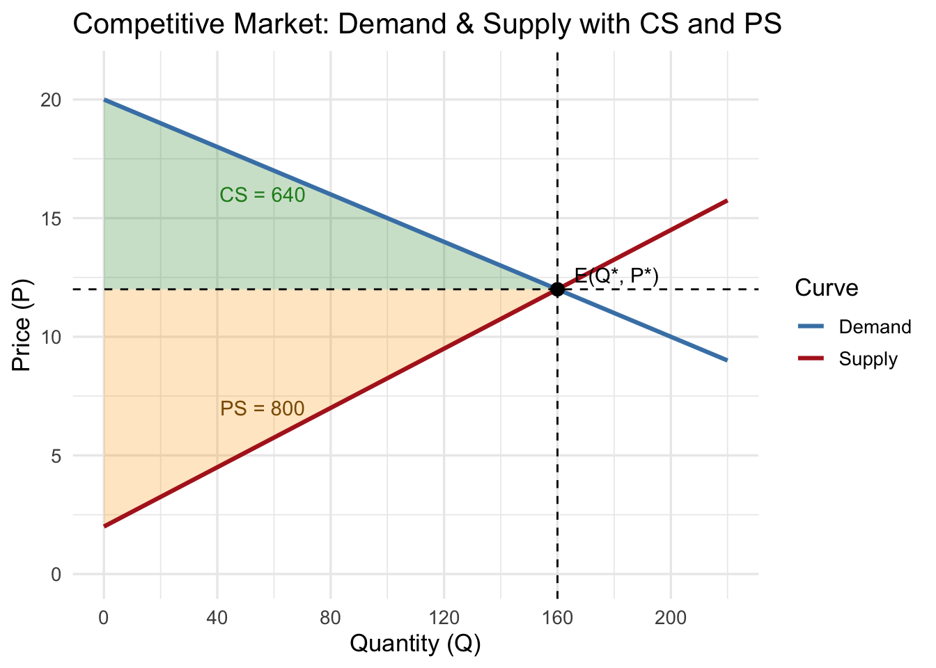
a. Draw the demand curve and the supply curve on the same graph. Clearly label both curves.
b. Solve for the equilibrium price and equilibrium quantity.
c. Calculate the numerical values of consumer surplus (CS) and producer surplus (PS).
d. On your graph, shade and label the areas corresponding to CS and PS.
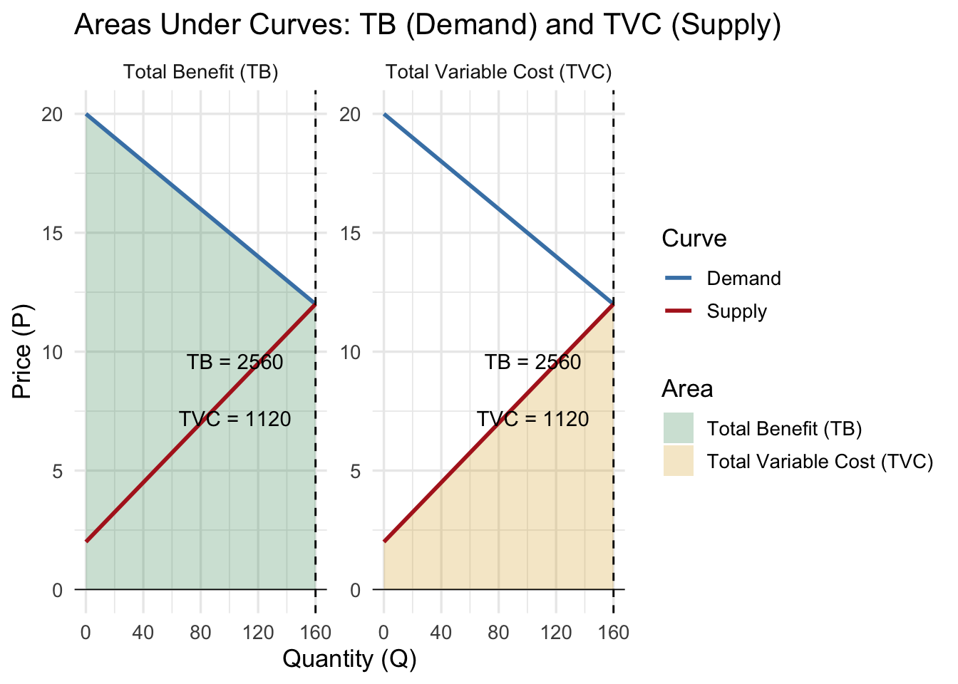
e. Compute the total benefit (TB) for the equilibrium quantity and the total variable cost (TVC) of supplying that quantity. Indicate these areas on your graph.

Show answer

We are given:

\[ \begin{align} Q_D &= 400 - 20P \\ Q_S &= 16P - 32 \end{align} \] This is equivalent to:

\[ \begin{align} MB(Q) &= 20 - \frac{1}{20}Q \\ MC(Q) &= \frac{1}{16}Q + 2 \end{align} \]

1️⃣ Solve for Equilibrium

At equilibrium, \(Q_D = Q_S\):

\[ 400 - 20P = 16P - 32 \]

\[ 432 = 36P \Rightarrow P^* = 12 \]

Substitute \(P^* = 12\) into either equation:

\[ Q^* = 400 - 20(12) = 160 \]

Thus,
Equilibrium Price: \(P^* = 12\)
Equilibrium Quantity: \(Q^* = 160\)

---

2️⃣ Compute Surpluses and Totals

• Demand intercept (where \(Q_D = 0\)):
  \(400 - 20P = 0 \Rightarrow P = 20\)

• Supply intercept (where \(Q_S = 0\)):
  \(16P - 32 = 0 \Rightarrow P = 2\)

Then:

\[ CS = \tfrac{1}{2}(P_{max} - P^*)Q^* = \tfrac{1}{2}(20 - 12)(160) = 640 \]

\[ PS = \tfrac{1}{2}(P^* - P_{min})Q^* = \tfrac{1}{2}(12 - 2)(160) = 800 \]

Total Benefit (area under demand curve up to \(Q^*\)):

\[ TB = \frac{1}{2}(20 + 12)\times 160 = 2560 \]

Total Variable Cost (area under supply curve up to \(Q^*\)):

\[ TVC = \frac{1}{2}(2 + 12)\times 160 = 1120 \]