Classwork 4
Optimal Harvesting in a Common-pool Fishery
Consider a fishery where the total benefit (TB) and total cost (TC) of fishing effort \(E\) are:
- \(TB(E)=1.5E - E^{2}\) (in $)
- \(TC(E)=0.5E\) (in $)
where \(E\) is the level of fishing effort (e.g., number of boat-days).
Key Concepts
Before beginning, recall these definitions:
Average Benefit (AB):
\(AB(E) = \dfrac{TB(E)}{E}\).
In economics, AB measures benefit per unit of input; here, it shows the revenue per boat-day.
For this fishery: \(AB(E) = \dfrac{1.5E - E^2}{E} = 1.5 - E\).Average Cost (AC):
\(AC(E) = \dfrac{TC(E)}{E}\).
In economics, AC measures cost per unit of input; here, it is the cost per boat-day.
For this fishery: \(AC(E) = \dfrac{0.5E}{E} = 0.5\).Marginal Benefit (MB):
\(MB(E) = \dfrac{dTB}{dE}\).
In economics, MB is the extra benefit from one more unit of input; here, the additional revenue from one more boat-day.
For this fishery: \(MB(E) = 1.5 - 2E\).Marginal Cost (MC):
\(MC(E) = \dfrac{dTC}{dE}\).
In economics, MC is the extra cost from one more unit of input; here, the additional cost of adding one boat-day.
For this fishery: \(MC(E) = 0.5\).
Benefit–Cost Table
Benefit–Cost Table
| Effort \(E\) |
TB \(1.5E - E^2\) |
MB \(1.5 - 2E\) |
AB \(1.5 - E\) |
TC \(0.5E\) |
MC \(0.5\) |
AC \(0.5\) |
|---|---|---|---|---|---|---|
| 0.05 | 0.073 | 1.400 | 1.450 | 0.025 | 0.500 | 0.500 |
| 0.10 | 0.140 | 1.300 | 1.400 | 0.050 | 0.500 | 0.500 |
| 0.15 | 0.202 | 1.200 | 1.350 | 0.075 | 0.500 | 0.500 |
| 0.20 | 0.260 | 1.100 | 1.300 | 0.100 | 0.500 | 0.500 |
| 0.25 | 0.312 | 1.000 | 1.250 | 0.125 | 0.500 | 0.500 |
| 0.30 | 0.360 | 0.900 | 1.200 | 0.150 | 0.500 | 0.500 |
| 0.35 | 0.402 | 0.800 | 1.150 | 0.175 | 0.500 | 0.500 |
| 0.40 | 0.440 | 0.700 | 1.100 | 0.200 | 0.500 | 0.500 |
| 0.45 | 0.473 | 0.600 | 1.050 | 0.225 | 0.500 | 0.500 |
| 0.50 | 0.500 | 0.500 | 1.000 | 0.250 | 0.500 | 0.500 |
| 0.55 | 0.522 | 0.400 | 0.950 | 0.275 | 0.500 | 0.500 |
| 0.60 | 0.540 | 0.300 | 0.900 | 0.300 | 0.500 | 0.500 |
| 0.65 | 0.552 | 0.200 | 0.850 | 0.325 | 0.500 | 0.500 |
| 0.70 | 0.560 | 0.100 | 0.800 | 0.350 | 0.500 | 0.500 |
| 0.75 | 0.562 | 0.000 | 0.750 | 0.375 | 0.500 | 0.500 |
| 0.80 | 0.560 | -0.100 | 0.700 | 0.400 | 0.500 | 0.500 |
| 0.85 | 0.552 | -0.200 | 0.650 | 0.425 | 0.500 | 0.500 |
| 0.90 | 0.540 | -0.300 | 0.600 | 0.450 | 0.500 | 0.500 |
| 0.95 | 0.522 | -0.400 | 0.550 | 0.475 | 0.500 | 0.500 |
| 1.00 | 0.500 | -0.500 | 0.500 | 0.500 | 0.500 | 0.500 |
| 1.05 | 0.473 | -0.600 | 0.450 | 0.525 | 0.500 | 0.500 |
| 1.10 | 0.440 | -0.700 | 0.400 | 0.550 | 0.500 | 0.500 |
| 1.15 | 0.402 | -0.800 | 0.350 | 0.575 | 0.500 | 0.500 |
| 1.20 | 0.360 | -0.900 | 0.300 | 0.600 | 0.500 | 0.500 |
| 1.25 | 0.312 | -1.000 | 0.250 | 0.625 | 0.500 | 0.500 |
| 1.30 | 0.260 | -1.100 | 0.200 | 0.650 | 0.500 | 0.500 |
| 1.35 | 0.202 | -1.200 | 0.150 | 0.675 | 0.500 | 0.500 |
| 1.40 | 0.140 | -1.300 | 0.100 | 0.700 | 0.500 | 0.500 |
| 1.45 | 0.073 | -1.400 | 0.050 | 0.725 | 0.500 | 0.500 |
| 1.50 | 0.000 | -1.500 | 0.000 | 0.750 | 0.500 | 0.500 |
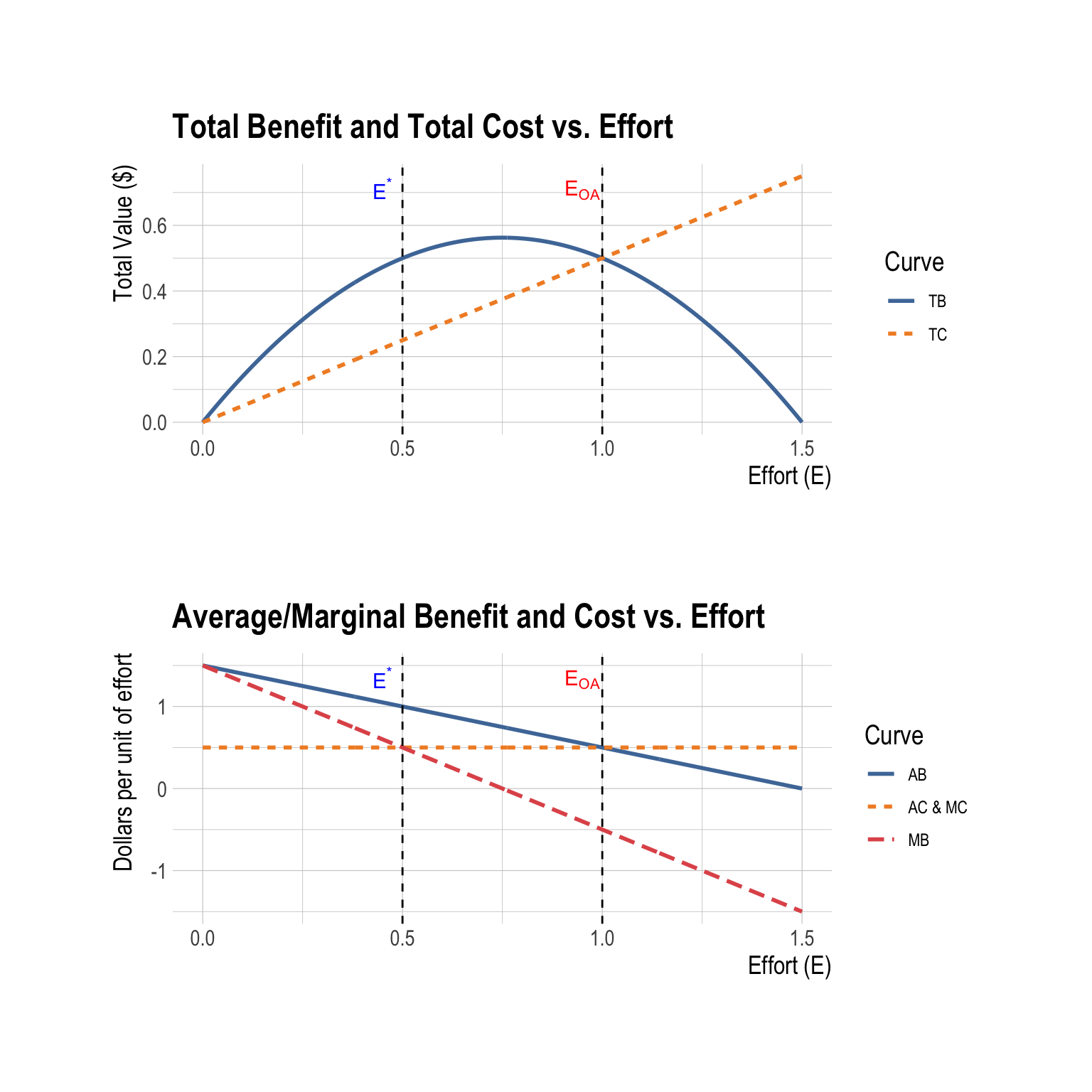
Part A — Total Curves
Draw the Total Benefit (TB) and Total Cost (TC) curves as functions of fishing effort \(E\). Place these curves in the top panel of a two-panel figure.
Part B — Marginal Curves
On the bottom panel, draw the Marginal Benefit (MB) and Marginal Cost (MC) curves as functions of fishing effort \(E\).
Part C — Efficient and Open-Access Effort Levels
Make sure the top and bottom panels share the same horizontal scale for effort \(E\), so the relationship between total and marginal spaces is consistent.
- Recall that:
- \(MB(E)=\dfrac{d\,TB}{dE}=1.5 - 2E\)
- \(MC(E)=\dfrac{d\,TC}{dE}=0.5\)
On both panels, mark and label the two benchmark effort levels using vertical guide lines that align across panels:
The efficient effort \(E^*\): Draw a vertical line at \(E^*\) on both the top (TB/TC) and bottom (AB/AC/MB/MC) panels and label it “\(E^*\)”.
The open-access effort \(E_{OA}\): Draw a vertical line at \(E_{OA}\) on both panels and label it “\(E_{OA}\)”.
Show answer
Part D — Intuition Behind \(E^*\) and \(E_{OA}\)
Explain the intuition behind these two effort levels:
- Why does \(E^*\) arise?
- Why does \(E_{OA}\) arise under open access?
Show answer
Efficient Effort (\(E^*\))
- The efficient effort arises where the marginal benefit (MB) from fishing equals the marginal cost (MC) of fishing.
- At this point, the last unit of effort adds just as much value as it costs to provide.
- Any increase in effort beyond \(E^*\) would add less benefit than cost, reducing total economic welfare.
- Thus, \(E^*\) represents the socially optimal level of effort that maximizes net economic benefit (total benefit − total cost).
Open-Access Effort (\(E_{OA}\))
- Under open access, anyone can freely enter the fishery until profits are driven to zero.
- Entry continues until the average benefit (AB) equals the average cost (AC) — meaning fishers just break even, with no economic rent remaining.
- At \(E_{OA}\), total effort exceeds the efficient level \(E^*\) because individual fishers ignore how their effort affects others and the fish stock.
- This leads to overfishing and rent dissipation, known as the “tragedy of the commons.”
Part E — Policy Intervention with a License Fee
- License fee: Explain, both analytically and intuitively, how charging a license fee (e.g., license fee per boat-day) can reduce fishing effort from the open-access level \(E_{OA}\) down to the efficient level \(E^*\).
- Explain why it is important to align individual fishers’ incentives with the socially optimal level of effort in a fishery. In your answer, discuss:
- Incentive problem: Why do individual fishers’ private decisions differ from what is best for the group?
- Economic rent: What happens to economic rents under open access when incentives are not aligned?
- Sustainability: Why does aligning incentives matter for the long-run health of both the fish stock and the fishing economy?
Show answer
- Analytically: A per-unit license fee raises each fisher’s private cost of fishing effort. This shifts the AC/MC curve upward, so that the new open-access equilibrium occurs at a lower effort level. The fee can be set so that the new equilibrium aligns exactly with the efficient level \(E^*\).
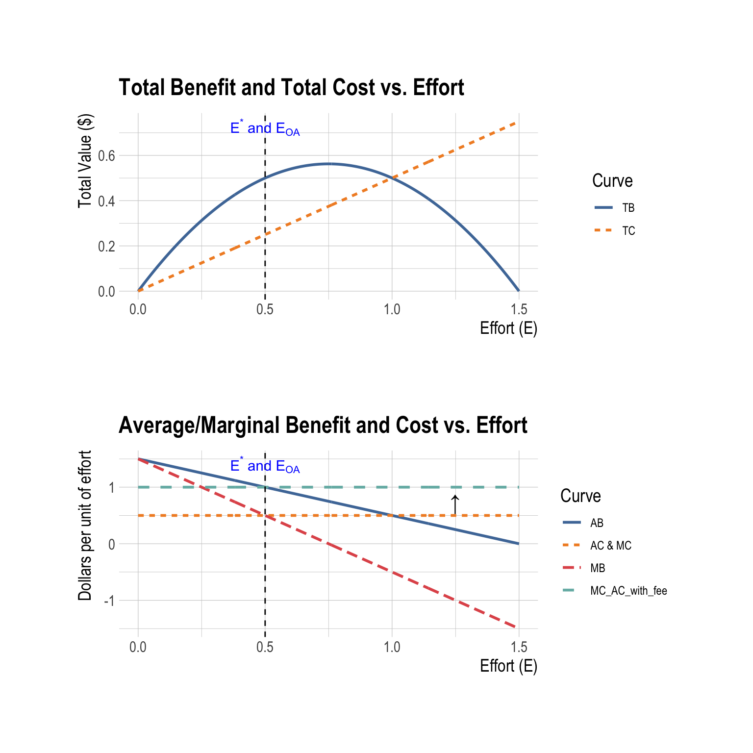
Intuitively: By making it more expensive to fish, the license fee discourages excessive entry. Only fishers whose effort generates enough value to cover the fee will remain, cutting effort back to the socially optimal level.
Why aligning incentives is crucial
- Incentive problem: Individual fishers decide based on their own costs and benefits, ignoring the fact that their fishing reduces the stock for others. This leads to effort beyond the social optimum.
- Economic rent: When incentives are misaligned under open access, economic rents are dissipated—profits vanish as more boats chase fewer fish.
- Sustainability: Aligning private and social incentives ensures that the fish stock is not overharvested, protecting both the long-run ecological health of the fishery and the economic viability of the fishing community.