Homework 1
Externalities; EPA Edangerment Finding on GHG Emissions; Coase Theorem
Homework Instructions
No Generative AI: You are not allowed to use generative AI tools for Homework Assignment 1.
Deadlines:
- Questions 1, 3, and 4: Due Wednesday, September 24, 2025 at 10:30 A.M. (ET)
- Hand in your written answers on paper to Prof. Choe at the beginning of class.
- Hand in your written answers on paper to Prof. Choe at the beginning of class.
- Question 2: Due Monday, September 22, 2025 at 11:59 P.M.
- Submit your comment as a PDF or Word document on Brightspace.
- When uploading, please also leave a note in the submission box indicating whether you submitted your comment to the U.S. EPA.
- Submit your comment as a PDF or Word document on Brightspace.
- Questions 1, 3, and 4: Due Wednesday, September 24, 2025 at 10:30 A.M. (ET)
Question 1. Externalities and Economic Development (Points: 30)
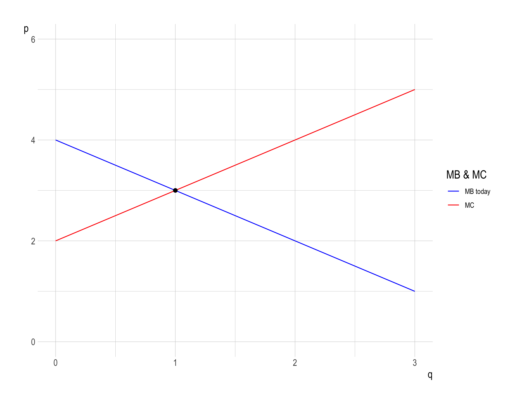
The demand function for oil is \(q_d = 4 - p\), and the supply function is \(q_s = p - 2\), where \(p\) is the price of oil per barrel, and \(q\) is the quantity of oil in millions of barrels per day. Using this information, solve the following problems:
a.
Graph the supply and demand functions on the same coordinate plane.
Show answer
b.
Determine the market equilibrium price and quantity of oil.
Show answer
- Solving the system of demand and supply equations gives the market equilibrium level of quantity (\(q_M\)) and price (\(p_M\)): \[ \begin{align} MB(q_M) =\; &p_M = MC(q_M)\\ 4 - q_M =\; &q_M + 2\\ \quad\\ \therefore\quad \left\{\begin{matrix} q_M = 1 \\ p_M = 3 \end{matrix}\right. \end{align} \]
c.
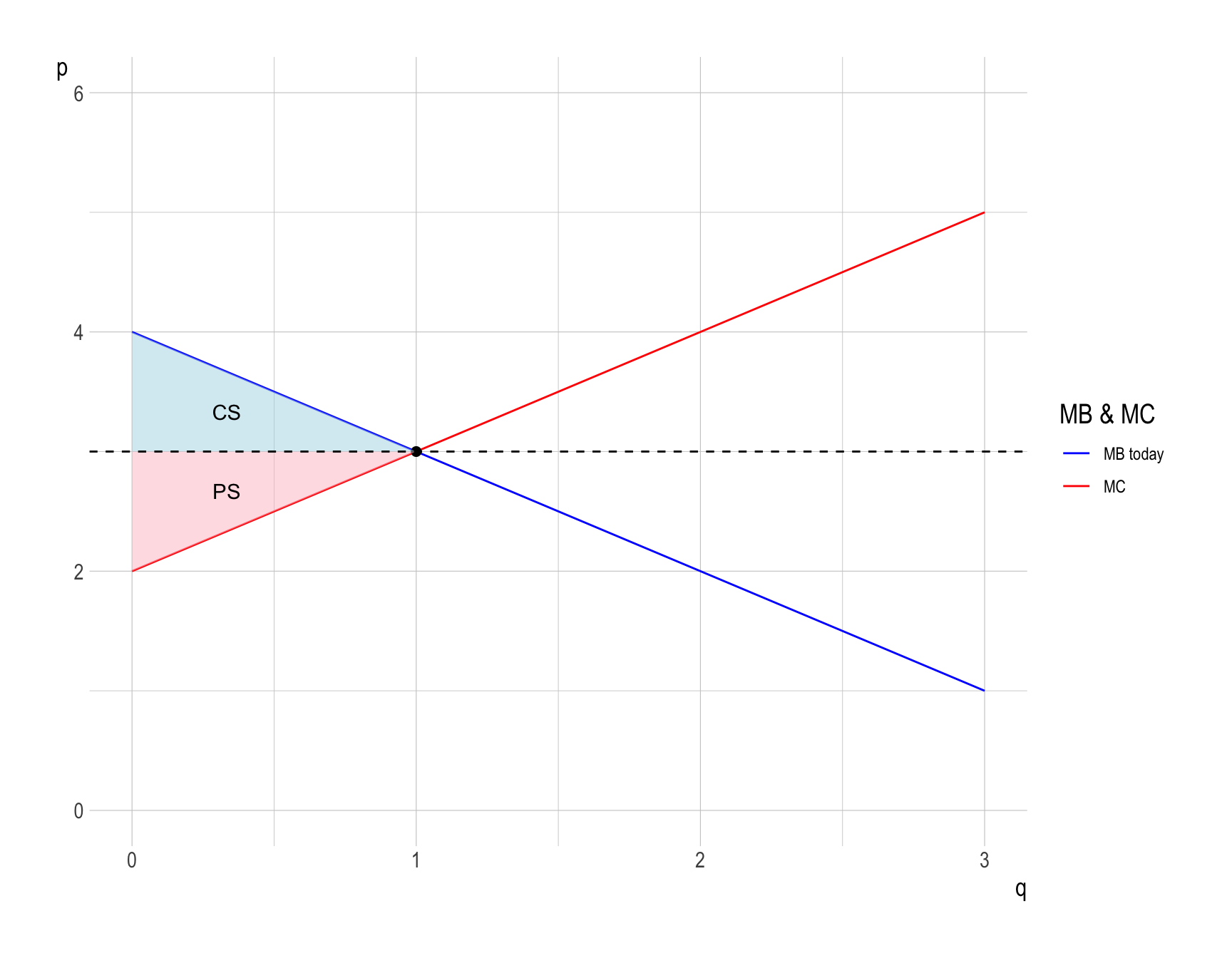
Calculate the consumer surplus and producer surplus at the market equilibrium.
Show answer
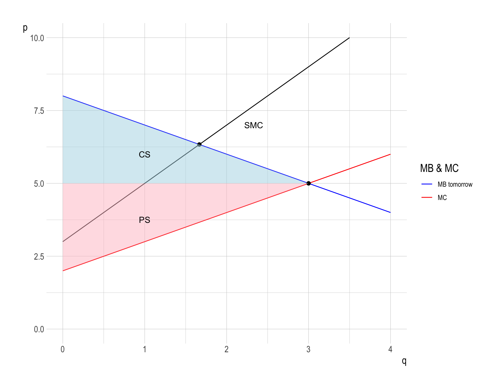
- Consumer surplus (\(CS\)) is the value that consumers receive from an allocation minus what it costs them to obtain it.
- \(CS\) is measured as the area under the demand curve minus the consumer cost.
- Producer surplus (\(PS\)) is the value that producers receive from an allocation minus what it costs them to supply it.
- \(PS\) is measured as the area above the supply curve and below the market price line.
- Therefore, \(CS = \frac{1}{2}\) and \(PS = \frac{1}{2}\).
d.
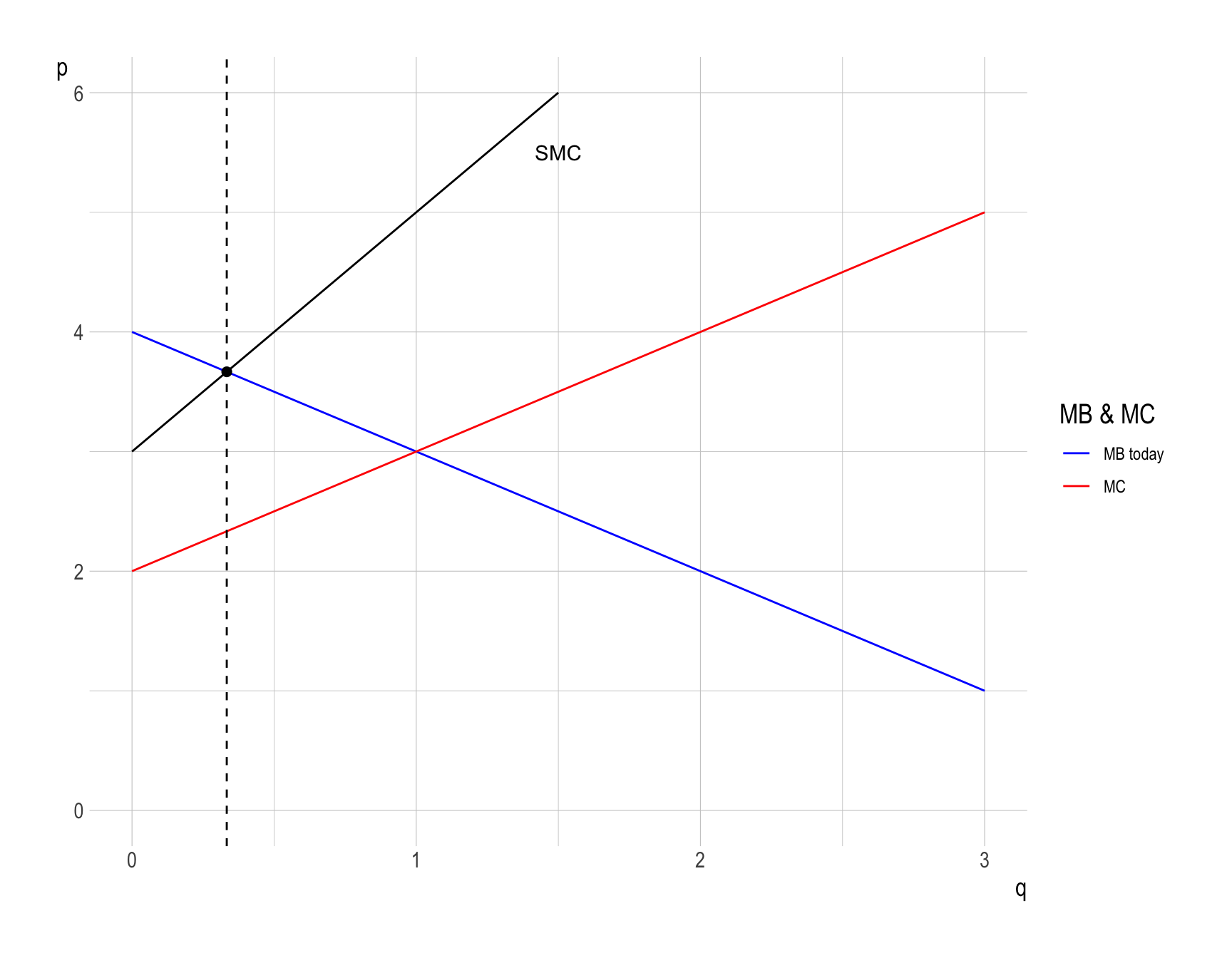
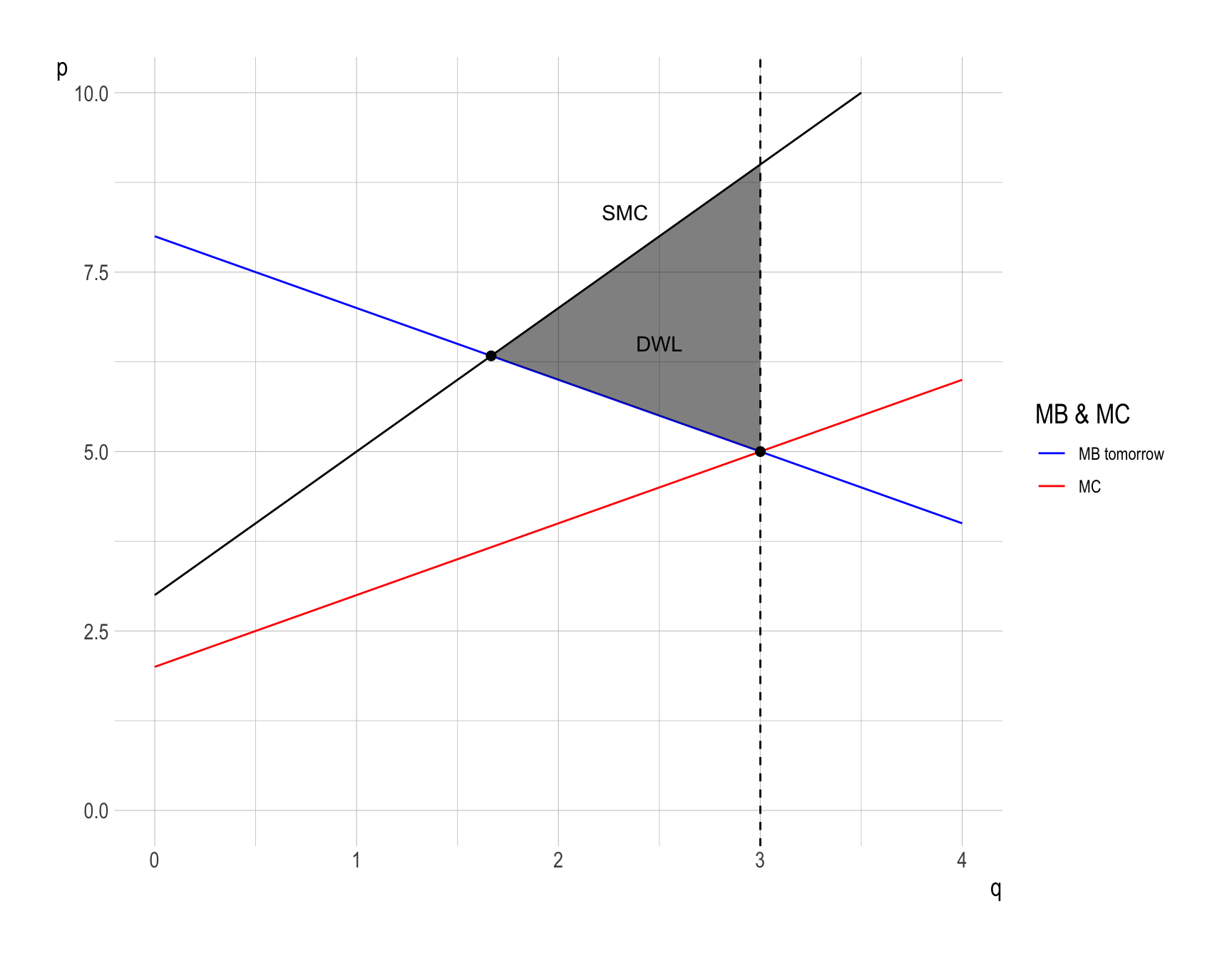
Oil consumption causes environmental damage. Suppose the external marginal cost of oil pollution is given by \(EMC = q + 1\). Calculate: (1) The socially optimal level of oil use (2) The deadweight loss due to pollution at the market equilibrium
Answer
(1) The socially optimal level of oil use
Show answer
The social marginal cost (\(SMC\)) is: \[ \begin{align} SMC &\,=\, EMC + MC\\ &\,=\, 2q + 3 \end{align} \] At the socially optimum \((q^{*}, p^{*})\), the social marginal cost of oil use is equal to the (social) marginal benefit:
\[ \begin{align} SMC &\,=\, MB\\ 2q^{*} + 3 &\,=\, 4 - q^{*} \end{align} \] Therefore, \(q^{*} = \frac{1}{3}\).
(2) The deadweight loss (\(DWL\)) due to pollution at the market equilibrium
Show answer
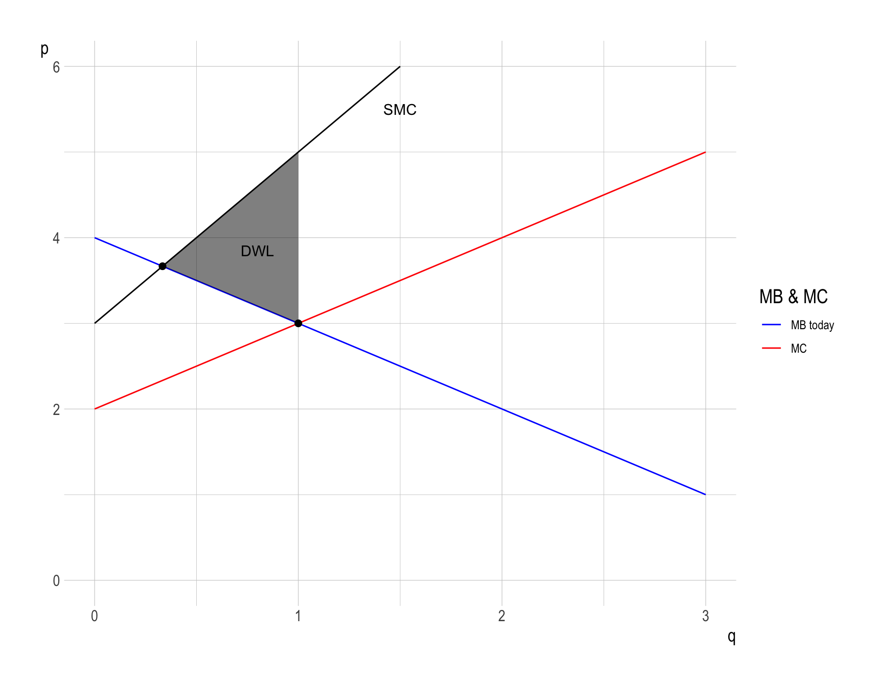
- Deadweight loss (\(DWL\)) is the loss of economic efficiency that occurs when the optimal or equilibrium outcome is not achieved in a market.
- What will happen if the firm produces at \(q_M\), instead of \(q^{*}\)?
- The total surplus (\(TS = CS + PS\)) is the same as in question (c).
- What will happen if the firm produces at \(q_M\), instead of \(q^{*}\)?
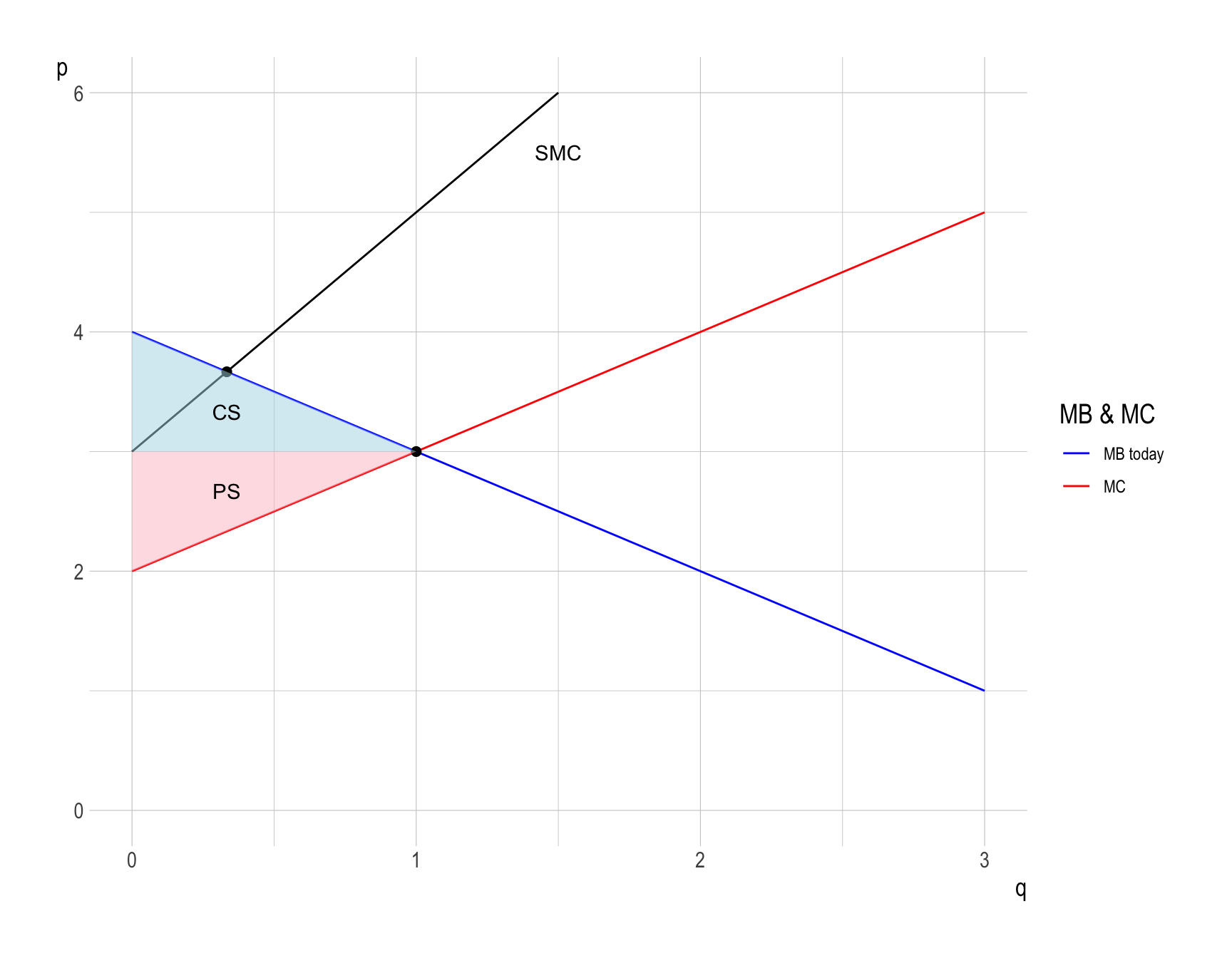
- However, pollution imposes a external total cost on society.
- This external cost is measured by the vertical distance between the Social Marginal Cost (\(SMC\)) and the Private Marginal Cost (\(MC\)) up to the production level \(q^{*} = 1\).
- Note that \(EMC = SMC - MC\).
- Imagine building up the external total cost unit by unit. For each unit of oil production, you add its marginal damage to society. The sum of all these marginal damage gives you the external total cost. Graphically, this summation is represented by the vertical distance between \(SMC\) and \(MC\).
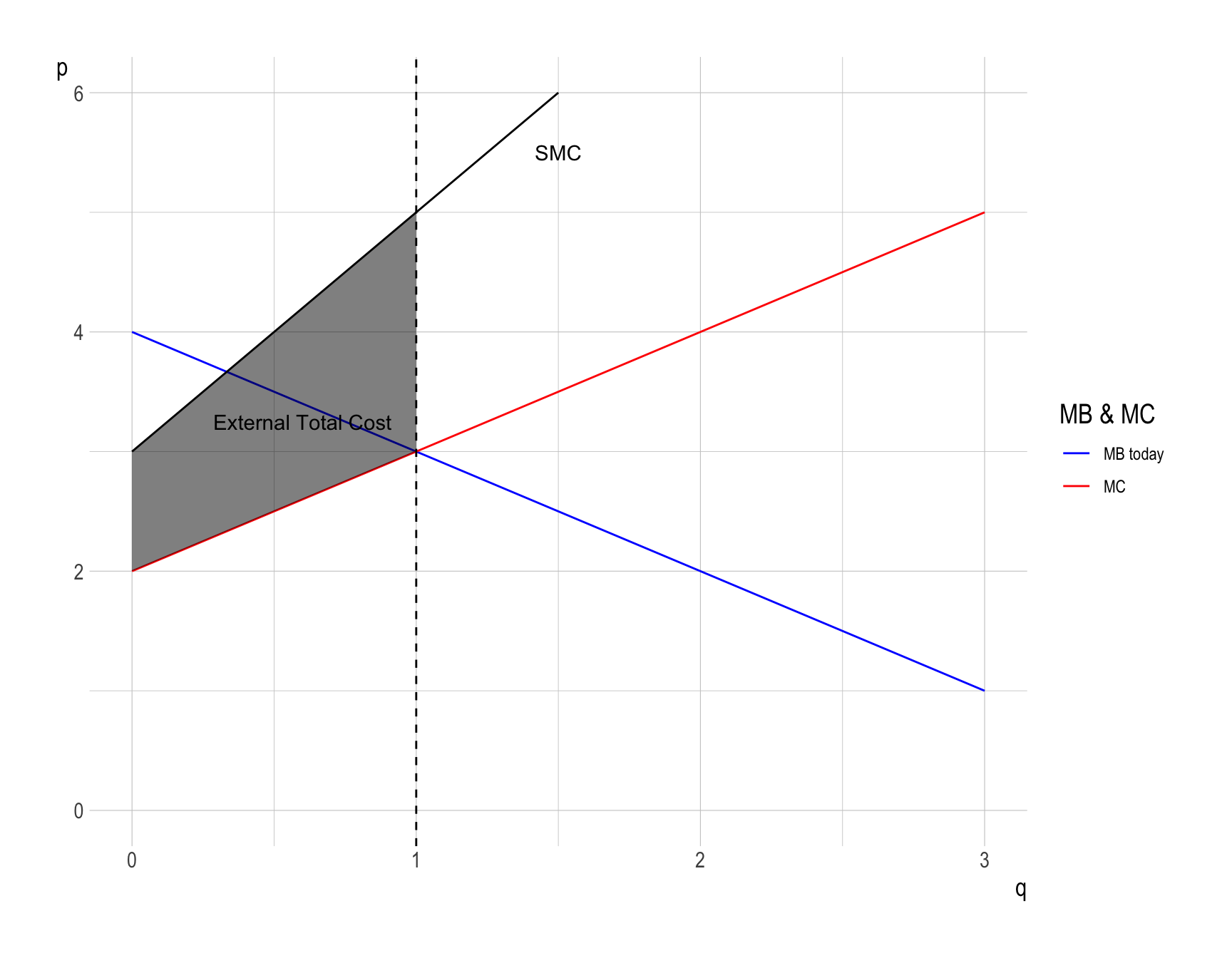
- Therefore, \(DWL\) can be calculated as the difference between the total surplus and the external total cost in the economy: \[ \begin{align} DWL &= \frac{1}{2}\times\left(1 - \frac{1}{3}\right)\times\left(5 - 3\right)\\ &= \frac{2}{3} \end{align} \]
e.
Due to economic development, the future demand for oil increases, resulting in a new demand function \(q_d' = 8 - p\). Determine: (1) The new market equilibrium price and quantity (2) The new socially optimal level of oil use (2) The deadweight loss due to pollution at the market equilibrium in the future
Answer:
(1) The new market equilibrium price and quantity
Show answer
In the equilibrium, the price is such that the market clears:
\[ 8 - q^{Future}_{M} = q^{Future}_{M} + 2 \] Therefore, the new equilibrium quantity is \(q^{Future}_{M} = 3\), and the new equilibrium price is \(p^{Future}_{M}=5\).
(2) The new socially optimal level of oil use
Show answer
At the new socially optimum \(q^{*Future}\), the social marginal benefit of the oil use is equal to the social marginal cost of the oil use:
\[ 8 - q^{*Future} = 2q^{*Future} + 3 \] Therefore, the new socially optimal level of oil use is \(q^{*Future} = \frac{5}{3}\).
(3) The \(DWL\) due to pollution at the market equilibrium in the future
Show answer
- Deadweight loss (\(DWL\)) is the loss of economic efficiency that occurs when the optimal or equilibrium outcome is not achieved in a market.
- What will happen if the firm produces at \(q^{Future}_{M}\), instead of \(q^{*Future}\)?
- The total surplus (\(TS = CS + PS\)) is described as below.
- What will happen if the firm produces at \(q^{Future}_{M}\), instead of \(q^{*Future}\)?
- However, producing at \(q^{Future}_{M} = 3\) creates the external total cost, the vertical distance between \(SMC\) and \(MC\)
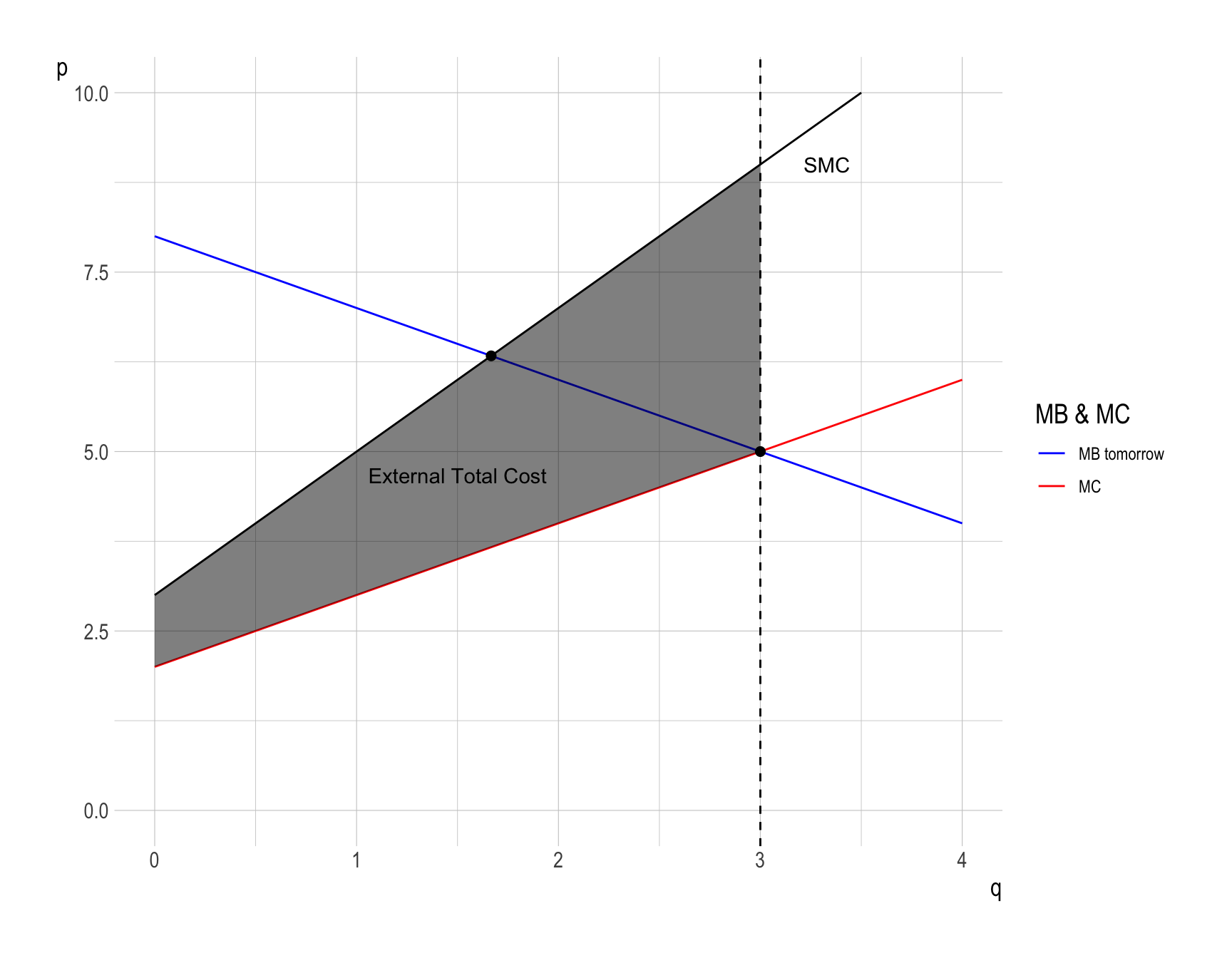
- Therefore \(DWL\) can be calculated as the difference between the total surplus and the external total cost in the market: \[ \begin{align} DWL &= \frac{1}{2}\times\left(3 - \frac{5}{3}\right)\times\left(9 - 5\right)\\ &= \frac{8}{3} \end{align} \]
f.
Propose and briefly explain two distinct public policies that could be implemented to mitigate the environmental damages and reduce the burden on future generations. Discuss the potential effectiveness and challenges of each policy.
Show answer
- Implement a Pigouvian Tax
- Policy: Impose a tax equal to the marginal external cost of pollution (e.g., a carbon tax).
- Benefits:
- Internalizes the environmental cost of pollution, incentivizing firms and consumers to reduce emissions
- Generates government revenue that can be reinvested in sustainability initiatives or used to offset regressive effects on low-income households
- Internalizes the environmental cost of pollution, incentivizing firms and consumers to reduce emissions
- Challenges:
- Determining the “correct” tax level can be politically and technically difficult
- Strong resistance from industries and consumers sensitive to price increases
- Determining the “correct” tax level can be politically and technically difficult
- Long-term Impact: Creates consistent market signals that encourage cleaner technologies and reduce environmental harm over time
- Policy: Impose a tax equal to the marginal external cost of pollution (e.g., a carbon tax).
- Direct Public Investment in Renewable Energy
- Policy: Government funds large-scale projects in solar, wind, and other renewable sources
- Benefits:
- Immediately expands the supply of clean energy, reducing reliance on fossil fuels
- Encourages innovation and job growth in the green sector
- Improves long-term energy security
- Immediately expands the supply of clean energy, reducing reliance on fossil fuels
- Challenges:
- Requires substantial upfront public spending, potentially straining budgets
- Must overcome fossil fuel infrastructure “lock-in” and opposition from incumbent industries
- Effectiveness depends on careful allocation to avoid waste or inefficiency
- Requires substantial upfront public spending, potentially straining budgets
- Long-term Impact: Accelerates the energy transition, lowering environmental damages and easing the burden on future generations by reducing climate risks
- Policy: Government funds large-scale projects in solar, wind, and other renewable sources
g.
Suppose the government decides to impose a Pigouvian tax to internalize the external costs of oil pollution. Calculate the optimal tax rates in the present and in the future and explain how it would affect the market equilibrium and social welfare.
Pigouvian Tax for Oil Production:
Show answer
- To address the negative externality imposed by oil production, we are considering implementing a price instrument known as Pigouvian tax, or corrective taxation. This policy involves setting a per-unit tax equal to the marginal environmental damage caused by oil production.
\[ \begin{align} \text{Present}:&\quad t^{*} = EMC(q^{*}) = q^{*} + 1\\ \text{Future}:&\quad t^{*Future} = EMC(q^{*Future}) = q^{*Future} + 1 \end{align} \] - Therefore, the Pigouvian tax rate in the present is \(t^{*} = \frac{4}{3}\), and the Pigouvian tax in the future is \(t^{*Future} = \frac{8}{3}\).
How the Pigouvian Tax would affect the market equilibrium and social welfare
Show answer
Purpose of the Pigouvian Tax
The tax is designed to internalize the external costs of oil pollution by aligning private costs with social costs. Under this scheme, the Social Marginal Cost (SMC) curve becomes the effective private marginal cost of firms.
1. Optimal Tax Rates
- Present: The optimal tax equals the current external marginal cost of oil pollution.
- Future: The optimal tax should be updated to reflect future external damages, which may rise if pollution accumulates or environmental sensitivity increases.
2. Effect on Market Equilibrium
- The supply curve shifts upward by the tax amount.
- The new equilibrium has:
- A higher market price
- A lower equilibrium quantity
- A higher market price
- The burden of the tax is shared between producers and consumers, depending on the relative elasticities of demand and supply.
4. Long-Run Impacts
- Creates incentives for innovation in cleaner technologies and greater energy efficiency.
- Encourages substitution toward renewable energy and reduces long-term environmental damages.
5. Implementation Challenges
- Measurement: Difficulties in estimating the precise marginal external damage to set the correct tax.
- Economic Impact: Oil-dependent industries and regions may face adjustment costs.
- Political Resistance: Strong opposition likely from oil producers, consumers, and lobbyists.
- Equity Concerns: Higher energy prices can disproportionately affect lower-income households, requiring compensatory measures (e.g., rebates, targeted subsidies).
Question 3. Coase Theorem (Points: 30)
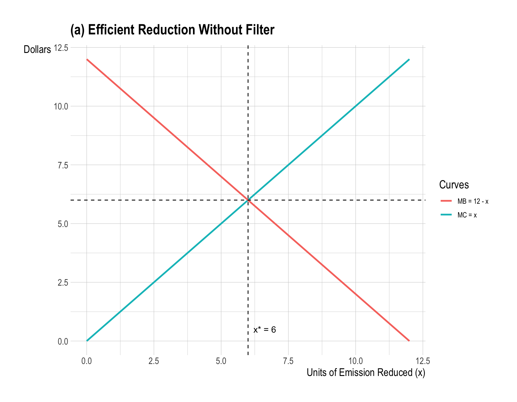
A small town has two factories, Alpha and Beta, located side by side. Alpha emits smoke that drifts into Beta’s building, making it harder for Beta’s workers to breathe and lowering their productivity. Currently, Alpha produces 12 units of smoke per day. Cutting back on emissions is costly:
Let \(x\) denote the units of emission reduced by Alpha (abatement). Treat \(x\) as any number from 0 to 12.
- Alpha’s marginal cost of reducing each unit of smoke is: \(MC = x\) (in $).
- Beta’s marginal benefit from each unit of reduction (cleaner air, healthier workers, higher productivity) is: \(MB = 12 − x\) (in $).
Two technological solutions are available:
- Beta can pay $10 per day to rent an air filter from a third party, which reduces Alpha’s smoke and improves the air quality in Beta’s workplace.
- Alpha can be relocated to another industrial site at a cost of $40 per day, which eliminates all exposure for Beta.
a.
Draw a diagram with “units of emission reduced” on the horizontal axis, showing marginal costs and marginal benefits. Without the filter or relocation, what is the efficient amount of smoke Alpha should cut?
Show answer
Set \(MC=MB\): \[ x = 12 - x \;\Rightarrow\; 2x=12 \;\Rightarrow\; \boxed{x^{*}=6}. \]
b.
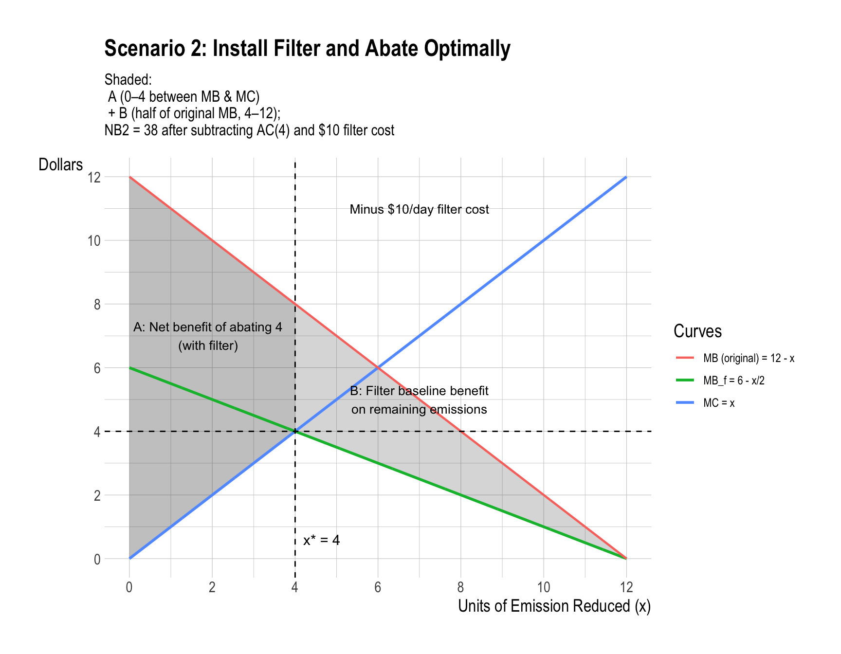
Suppose the air filter is installed, reducing Beta’s marginal benefit from each unit of abatement to \(\left(6 - \tfrac{x}{2}\right)\). That is, Beta now values emission reduction at only half the original level. What is the new efficient level of emission reduction?
Show answer
The filter halves Beta’s marginal benefit: \[ MB_f(x)=\tfrac{1}{2}(12-x)=6-\tfrac{x}{2}. \]
Set \(MC=MB_f\): \[ x = 6 - \frac{x}{2} \;\Rightarrow\; \frac{3}{2}x=6 \;\Rightarrow\; \boxed{x_f^{*}=4}. \]
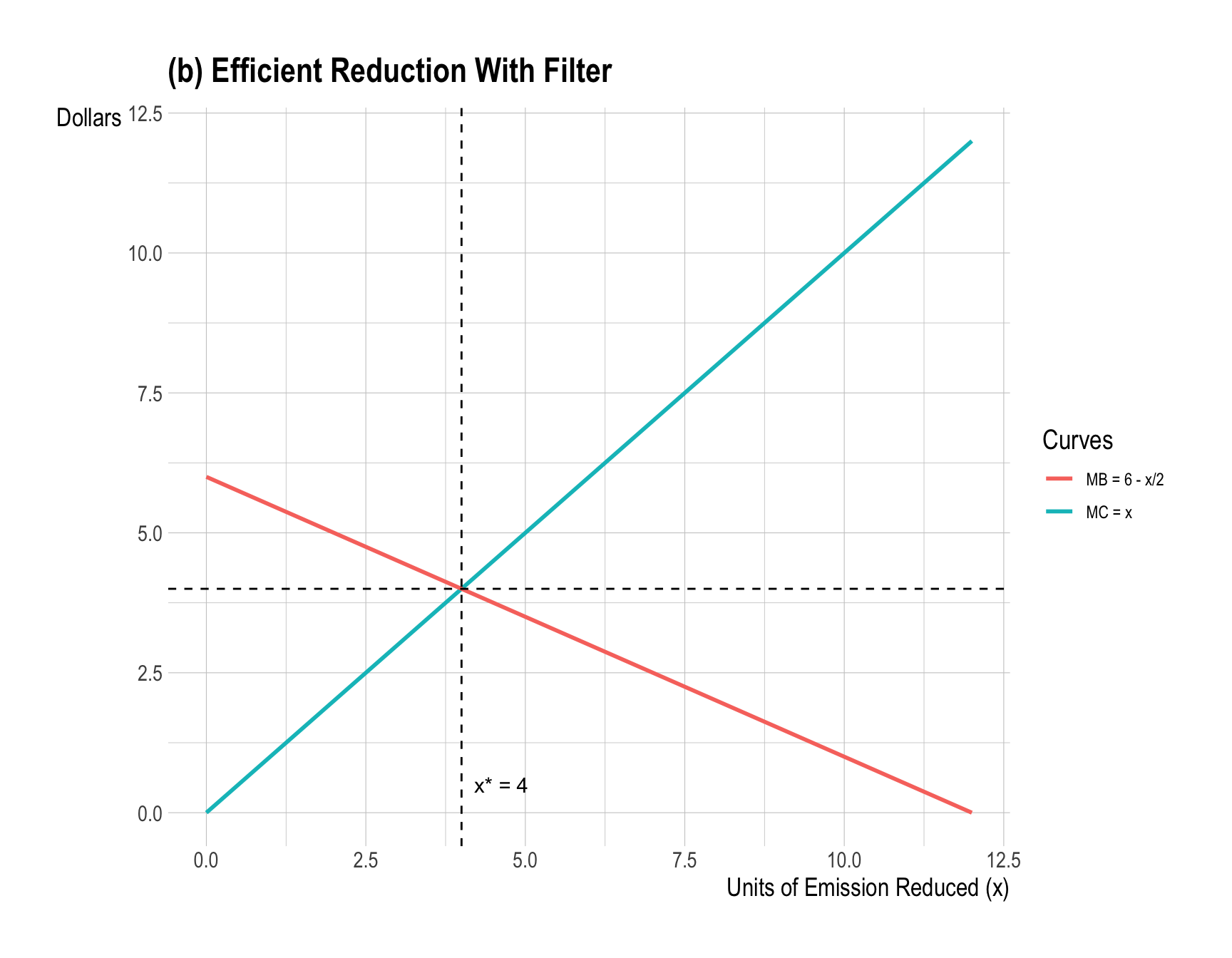
Why the Filter Halves Beta’s Marginal Benefit
- Without the filter:
Every unit of abatement removes 1 full unit of smoke.- If Alpha cuts back 1 more unit, Beta enjoys the full relief of that unit.
- The marginal benefit starts high (12) and declines linearly as fewer units remain:
\[ MB(x) = 12 - x \]
- If Alpha cuts back 1 more unit, Beta enjoys the full relief of that unit.
- With the filter:
The filter already removes half the harm from every unit of smoke that remains.- Each unit of abatement by Alpha now only solves half as much of a problem as before.
- Example: abating 1 unit takes Beta from “½ unit of smoke” to “0 smoke,” not from “1 full unit” to “0.”
- Each unit of abatement by Alpha now only solves half as much of a problem as before.
- Result:
Both the intercept and the slope of the MB curve are halved:
\[ MB_f(x) = \tfrac{1}{2}(12 - x) = 6 - 0.5x \]
The filter is already doing half the cleanup, so Beta values any additional abatement by Alpha at only half the original amount.
c.
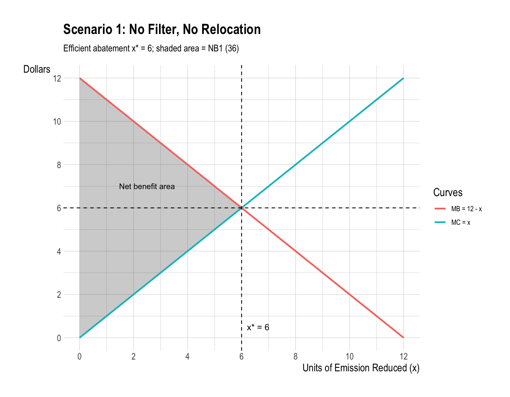
Calculate the net benefit (efficiency) of Beta for each scenario:
1. Do not rent the air filter or relocate Alpha, but instead pay Alpha not to emit smoke.
2. Rent the air filter and then also pay Alpha not to emit smoke.
(*Hint: There are two benefits under this scenario—(1) Relative to the status quo of 12 smoke emissions, the benefits of air filter rental have two components. First, Beta gets the full benefits of seeing 4 smoke reduced. Second, each unit of damage to Beta is cut in half by the filter for the remaining 8 smoke emissions.)
3. Pay to relocate Alpha.
Which scenario yields the highest efficiency? Show your calculations.
🔎 Guidelines:
- The net benefit (efficiency) is:
\[
(\text{Total Benefits from reduction}) \; - \; (\text{Total Costs (abatement + filter/relocation)})
\]
Answer
Scenario 1. Do not rent the air filter or relocate Alpha, but instead pay Alpha not to emit smoke.
Show answer
Scenario 2. Rent the air filter and then also pay Alpha not to emit smoke.
Show answer
Intuition with an Example
Suppose 1 unit of smoke causes $10 of harm to Beta.
With the filter in place:
- If Alpha emits that unit, the filter cuts the harm in half, so Beta only suffers $5 of damage.
- If Alpha abates that unit (doesn’t emit it at all), Beta avoids the entire $10 of harm, not just the $5 that would remain after the filter.
- If Alpha emits that unit, the filter cuts the harm in half, so Beta only suffers $5 of damage.
👉 This shows why the benefit of abating the first few units should be measured using the original marginal benefit curve, (MB(x) = 12 - x), not the reduced curve.
- For units that are abated → use the old MB curve ((12 - x)), since those units vanish completely relative to the status quo (12 units of smoke without the filter).
- For units that are not abated → count only half of the old MB, since the filter reduces their damage by 50% relative to the status quo.
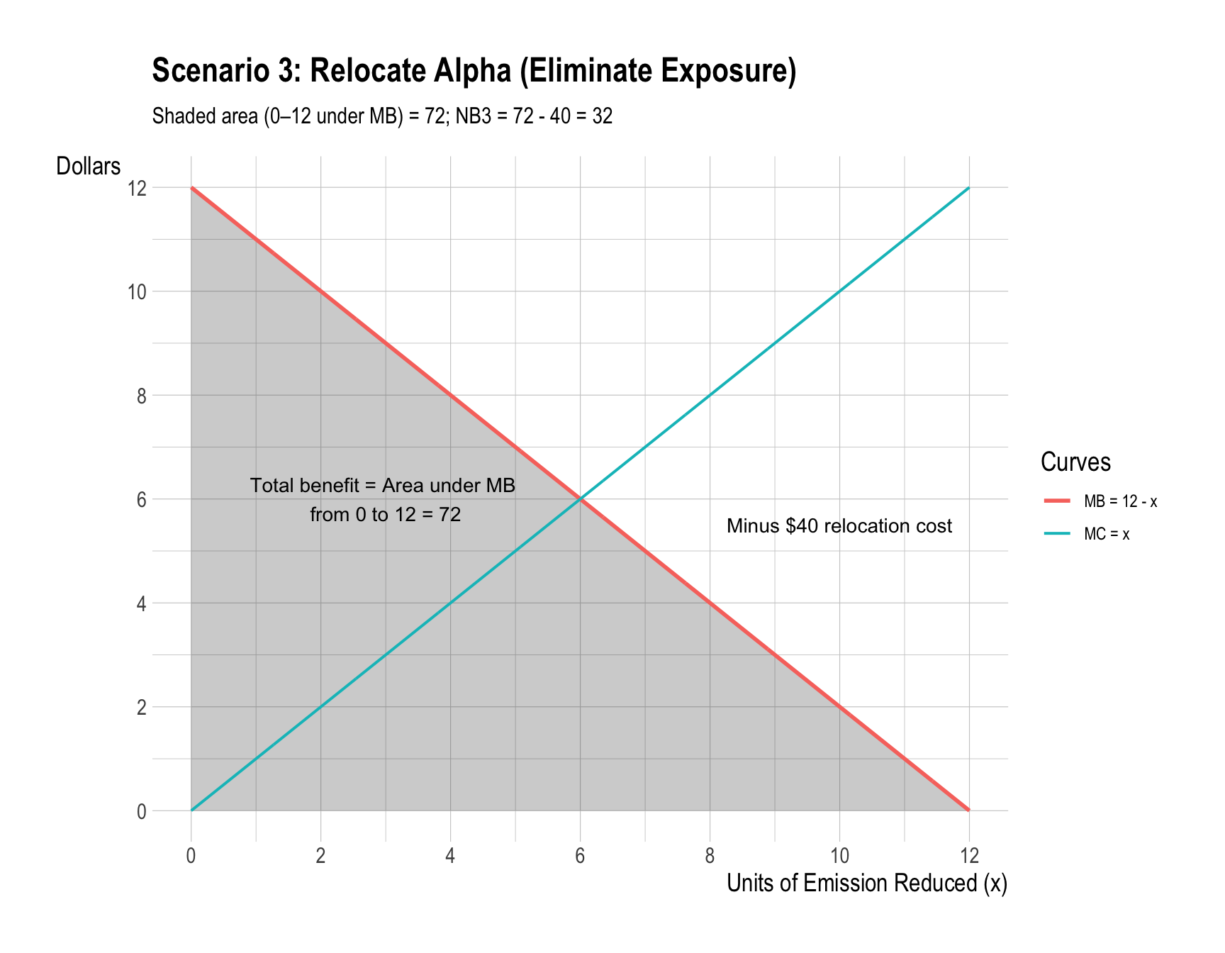
Scenario 3. Pay to relocate Alpha.
Show answer
Comparison & Conclusion
Show answer
\[ NB_1=36,\quad NB_2=38,\quad NB_3=32. \]
\[ \boxed{\text{Highest efficiency: Scenario 2 (filter + optimal abatement).}} \]
Implication of Scenario 2 (Filter + Abatement)
- With private negotiation, Beta and Alpha can agree to both install the filter ($10 per day) and abate 4 units.
- Even after including the filter’s fixed cost and Alpha’s abatement cost, this combined approach yields the highest net benefit compared with using only abatement or full relocation.
d.
Assume no transaction costs or free riding. According to the Coase theorem, explain why the two factories could reach the efficient outcome through negotiation even if Beta has the right to force Alpha to move at its own expense.
Show answer
If negotiation is easy and property rights are clear, Alpha and Beta can always reach the efficient outcome, no matter who holds the rights.
In this case, Scenario 2—installing the filter and reducing emissions by 4 units—gives the highest net benefit.
Key Lesson: The most effective solution often comes from a combination of technology and abatement. Through negotiation, both sides can agree on a plan that balances benefits, costs, and fixed expenses better than either extreme.
Note
Property rights determine who pays and who gains, but not the overall efficiency.
Question 2. EPA Endangerment Finding on Greenhouse Gas Emissions (Points: 40)
You have an opportunity to comment and voice your opinions on the US Environmental Protection Agency’s proposal to rescind its endangerment finding and end federal regulation of greenhouse gas emissions. Public comments on the proposal are invited and should be submitted no later than 11:59 PM EDT on Monday, September 22, 2025.
Homework Submission
For grading purposes, please submit a PDF of your comment to Brightspace by 11:59 PM EDT on Monday, September 22, 2025.
You are not required to submit your comment to the US EPA for grading. However, I strongly encourage you to take this opportunity to learn more about an important policy issue, practice your reasoning and argumentation skills, and engage in civic responsibility.
If you are not submitting your comment to the EPA, you do not need to include the docket ID or other identifying info from the “tips for effective comments.”
For this homework submission, there is no required font, spacing, citation style, or page format. Aim for about 2–3 pages if that is helpful, but shorter or longer is fine if your argument is clear and well-supported.
Please address the core question—whether GHGs should be treated as “air pollution” under CAA §202(a)—and take a clear position with reasoning and any sources you find useful.
How to Submit Comments to the US EPA
You can submit comments online or by email. The deadline for Submitting Comments is 11:59 PM EDT on Monday, September 22, 2025.
Commenting online:
- EPA prefers that comments be submitted online using the Federal eRulemaking Portal.
- Click this link for commenting on the EPA proposal, Docket ID No. EPA-HQ-OAR-2025-0194.
- Click the tab “Docket Documents.”
- Click the “Comment” button.
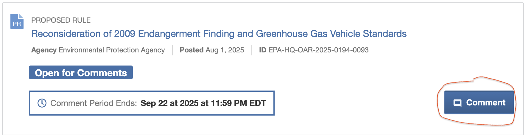
- Type or paste your comment in the comment field OR attach a file with your comment.
Commenting by Email:
- Type the Docket ID No. in the subject line of your email message: EPA-HQ-OAR-2025-0194
- Send your email to a-and-r-Docket@epa.gov.
Writing Effective Comments
Begin by informing yourself about EPA’s proposal, their analysis, and the analyses of others using links provided below. Search for additional credible sources.
Effective comments are concise and strongly reasoned. Recission of the endangerment finding will have many far-reaching consequences. Don’t attempt to be comprehensive in your comments; focus on one or two issues that are most salient to you. Support your comments with citations to sources if relevant. Include a statement about why the proposed recission is important to you personally. See also EPA’s tips for effective comments on rulemaking dockets.
Draft your comments using MS Word or similar program. This makes it easier for you to make and save revisions before you submit your comments.
The Main Issue: EPA’s Proposal to Reconsider the 2009 Endangerment Finding
Background
- 2009 Endangerment Finding: The EPA determined that greenhouse gases (GHGs) endanger public health and welfare, and that emissions from new motor vehicles contribute to this threat.
- Legal Foundation: This finding triggered the EPA’s obligation under Clean Air Act (CAA) §202(a) to regulate GHG emissions from cars and trucks.
- Supreme Court Ruling: In Massachusetts v. EPA (2007), the Court confirmed that GHGs are “air pollutants” under the Clean Air Act.
The Current Proposal (2025)
- EPA proposes to rescind the 2009 Endangerment Finding.
- This would remove the statutory basis for regulating GHG emissions from new vehicles under CAA §202(a).
- As a result, all GHG standards for light-, medium-, and heavy-duty vehicles would be repealed.
The Main Issue
Should GHGs be treated as “air pollution” under CAA §202(a), requiring EPA regulation, or not?
- Pro-Regulation View:
- GHGs clearly fit the Act’s definition of “air pollutant.”
- Vehicle emissions are a significant source of U.S. GHGs (~17% of total).
- Regulation delivers real emission cuts and large net economic benefits (fuel + maintenance savings, health co-benefits).
- Repeal View:
- Section 202(a) was not intended for global pollutants like CO₂.
- Vehicle standards have only a modest impact on global concentrations and warming.
- Compliance raises vehicle costs and limits consumer choice, creating economic harm.
Learn about EPA’s Proposal
Question 4. Class Participation (Not Graded for Homework 1)
Please write one sentence for each time you participated in class (any public speaking during class time) between August 25, 2025 and September 22, 2025.
Examples:
- “I asked a question to clarify the syllabus.”
- “I asked how carbon taxes affect consumer behavior.”
- “I gave plastic pollution as an example of a negative externality.”
- “I pointed out a calculation error during the lecture.”