The Economics of Wildfire Risk and Smoke

Reading for Lecture 8

A detailed reading on U.S. wildfire trends, wildfire risk, Canadian wildfire smoke in the eastern United States, decisions under risk, insurance markets, moral hazard, underinsurance, and recovery.

NoteConnection to Lecture 8

This reading follows the three classes of Lecture 8 and adds the sources, derivations, and caveats that the slides leave out. Read Sections 1 and 2 before Class 1, Section 3 before Class 2, and Sections 4 and 5 before Class 3. The textbook chapter is TL Chapter 12, Climate Change: Adaptation: Floods, Wildfires, and Water Scarcity, in Natural Resource Economics: The Essentials, 2nd edition. Kahn page numbers refer to the PDF of the June 2026 manuscript of An Introduction to Natural Disaster Economics.

More acres, not more fires

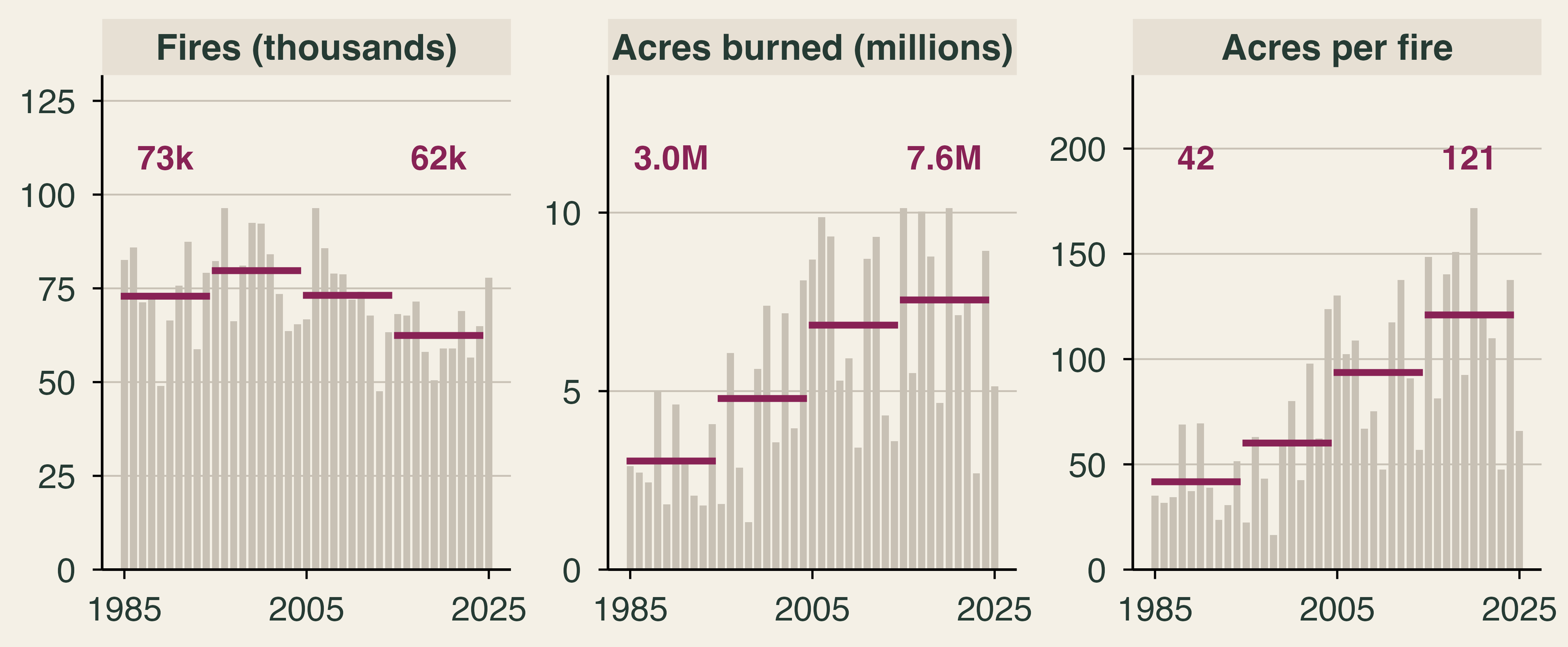
Why have wildfire losses climbed when the number of wildfires has not? Between 1985–94 and 2015–24, the average number of fires reported each year in the United States fell 14%, from about 73,000 to about 62,000. Acres burned moved the other way, from 3.0 million to 7.6 million a year. The average fire nearly tripled in size, from 42 acres to 121.

U.S. wildfire activity, 1985–2025. Bars show single years and lines show decade averages. Source: National Interagency Fire Center.

The National Interagency Fire Center (NIFC) counts every reported fire, including very small ones, so these averages understate how much large fires have changed. Satellite records point the same way: average fires in U.S. regions were up to four times larger and three times more frequent in the 2000s than in the two prior decades (Iglesias, Balch, and Travis, 2022). We start the series in 1985 because the 1983 and 1984 counts are about a quarter of the 1985 count, which looks like a reporting break rather than a real change. Single years are noisy: from 2024 to 2025, the number of fires rose 20% while acres burned fell 43%. Decade averages are the right unit for a trend.

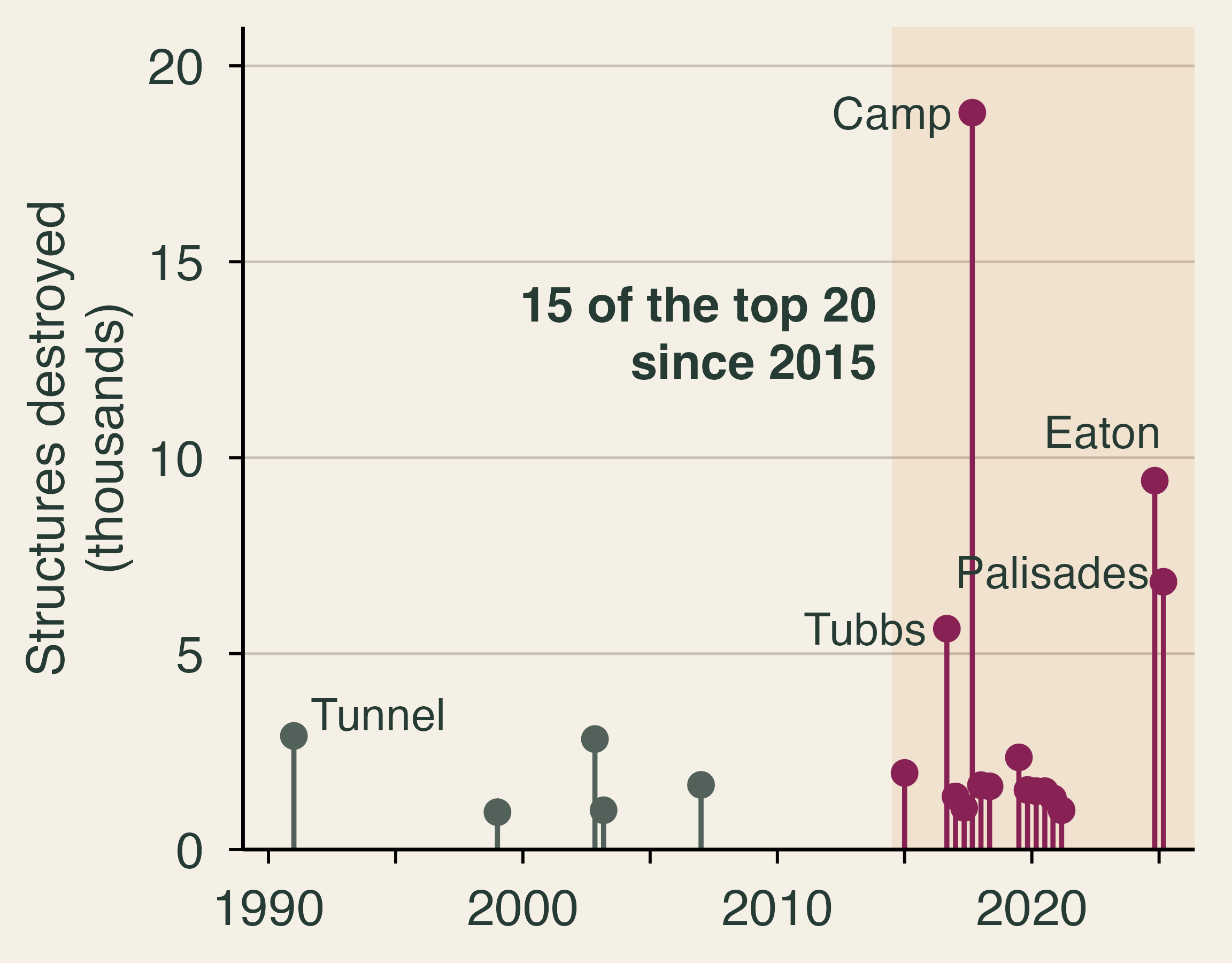
Acres are not damage. In 2025 the United States burned 5.1 million acres, 32% below the average of the previous ten years. Yet that year contained two of the three most destructive fires in California’s history. The Eaton and Palisades fires of January 2025 burned about 37,700 acres between them, less than 1% of the national total, and destroyed about 16,000 structures. Kahn (p. 144) puts the insured losses near $40 billion. Fifteen of California’s 20 most destructive fires have occurred since 2015, and seven of the top ten.

California’s 20 most destructive wildfires. Source: CAL FIRE, April 3, 2025. CAL FIRE marks the Eaton and Palisades counts as not final.

A fire becomes a disaster because of what it reaches, and in the eastern United States, what reaches people is often smoke rather than flame. Section 1 defines wildfire risk. Section 2 follows the smoke of Canada’s 2023 fire season to New York and the Great Lakes and asks how economists put a value on its damage. Section 3 shows how to make decisions when outcomes are uncertain. Section 4 examines insurance, and Section 5 turns to why people underprepare and who recovers.

1. From a fire to a disaster

Textbook reading. TL Chapter 12. Kahn, pp. 3–8, 15–16, 21–28, 83–84, and 95–96.

Hazard, exposure, and vulnerability

Wildfire risk comes from the interaction of three elements. Hazard is how likely and how intense a fire is. Exposure is who and what stands in its path. Vulnerability is how much harm the fire does when it arrives. Climate scientists define climate risk through the same three elements, and we can write the idea as

\text{Wildfire risk} \;\propto\; \text{Hazard} \times \text{Exposure} \times \text{Vulnerability}.

The product is a shorthand, and it makes one point well: if any element is zero, there is no loss. A large fire in empty wilderness is a hazard with no exposure. The product also tells us where policy can act. Fuel treatment works on hazard, land-use rules on exposure, building codes on vulnerability, and insurance on none of the three, because it moves the financial loss rather than shrinking the physical one.

All three elements have moved. On hazard, Abatzoglou and Williams (2016) estimate that human-caused climate change added 4.2 million hectares of forest fire area across the western United States during 1984–2015, nearly doubling what would have burned otherwise. Speed matters too. Balch et al. (2024) study more than 60,000 fires from 2001 to 2020 and call a fire “fast” if it grows more than 1,620 hectares (about 4,000 acres) in one day. Fast fires were 2.7% of all fires, yet they accounted for 78% of structures destroyed and 61% of suppression costs. A fire that moves that quickly leaves little time to evacuate or to defend homes.

On exposure, the number of houses in the wildland-urban interface, where homes meet or mix with undeveloped vegetation, rose from 30.8 million in 1990 to 43.4 million in 2010 (Radeloff et al., 2018). New housing, not new vegetation, explains 97% of the new interface area. Kahn calls this the “bull’s-eye effect” (p. 28): we keep adding homes, roads, and power lines in the places where fires burn. People do not choose these places for the risk. They buy a bundle of views, schools, weather, and jobs, and the risk comes attached (pp. 83–84). You met this idea in Lecture 7: a house price is the price of a bundle.

On vulnerability, the same fire can do very different damage. As reported in Kahn (pp. 95–96), post-fire inspections by the Insurance Institute for Business & Home Safety (IBHS) after the Los Angeles fires found that homes with multiple fire-resistant features had a 54% chance of no damage, compared with 36% for homes with fewer features. Each additional 10 feet between homes raised the odds of survival by 7% to 13%. Some steps are cheap: vent screens cost $100 to $500, and clearing fuel near a home costs $500 to $2,000. Owners also weigh costs that are not in dollars. Hardening can look worse, and clearing removes vegetation that owners like. These are comparisons rather than causal estimates, since homes with more features may differ in other ways, so Section 3 turns to stronger evidence.

Mitigation or adaptation?

The word “mitigation” means different things in different fields, and the difference matters for this lecture. In climate economics, mitigation means cutting greenhouse gas emissions. Its benefits are global, because a ton of carbon dioxide warms the planet no matter where it is emitted, and they arrive slowly. Adaptation means reducing the damage from the climate we get. Its benefits are local and arrive sooner. Fire agencies and many of the studies below call brush clearing and home hardening “mitigation,” but in climate economics those are adaptation. So is an air purifier bought for smoke season. Because some warming is locked in, we need both, and most of this lecture is about choosing among adaptation options.

Are disaster losses natural?

Kahn’s central claim is that disaster losses are endogenous: they emerge from choices shaped by incentives (p. 4). In his words, the damage “is not a law of physics” (p. 15). He applies this to Los Angeles, arguing that coastal land-use rules, Proposition 13, insurance price ceilings, and single-family zoning together served as the “kindling” (pp. 21–24). This is a causal argument, and Kahn presents his themes as hypotheses that evidence could reject (p. 16). As you read the studies below, ask which of his claims they support and which remain untested.

2. Smoke without borders

Textbook reading. Kahn, pp. 63–66, 114, and 186.

The flames of a wildfire stop at the burn perimeter, but the smoke does not. Fine particles smaller than 2.5 micrometers across (PM_2.5), about one-thirtieth the width of a human hair, can travel thousands of kilometers, lodge deep in the lungs, and pass into the bloodstream. For most people in the eastern United States, wildfire arrives as smoke rather than flame. This section follows one fire season, Canada’s in 2023, and uses it to develop four economic ideas: a transboundary externality, the value of a statistical life, defensive spending, and the unequal ability to defend.

Canada’s 2023 fire season

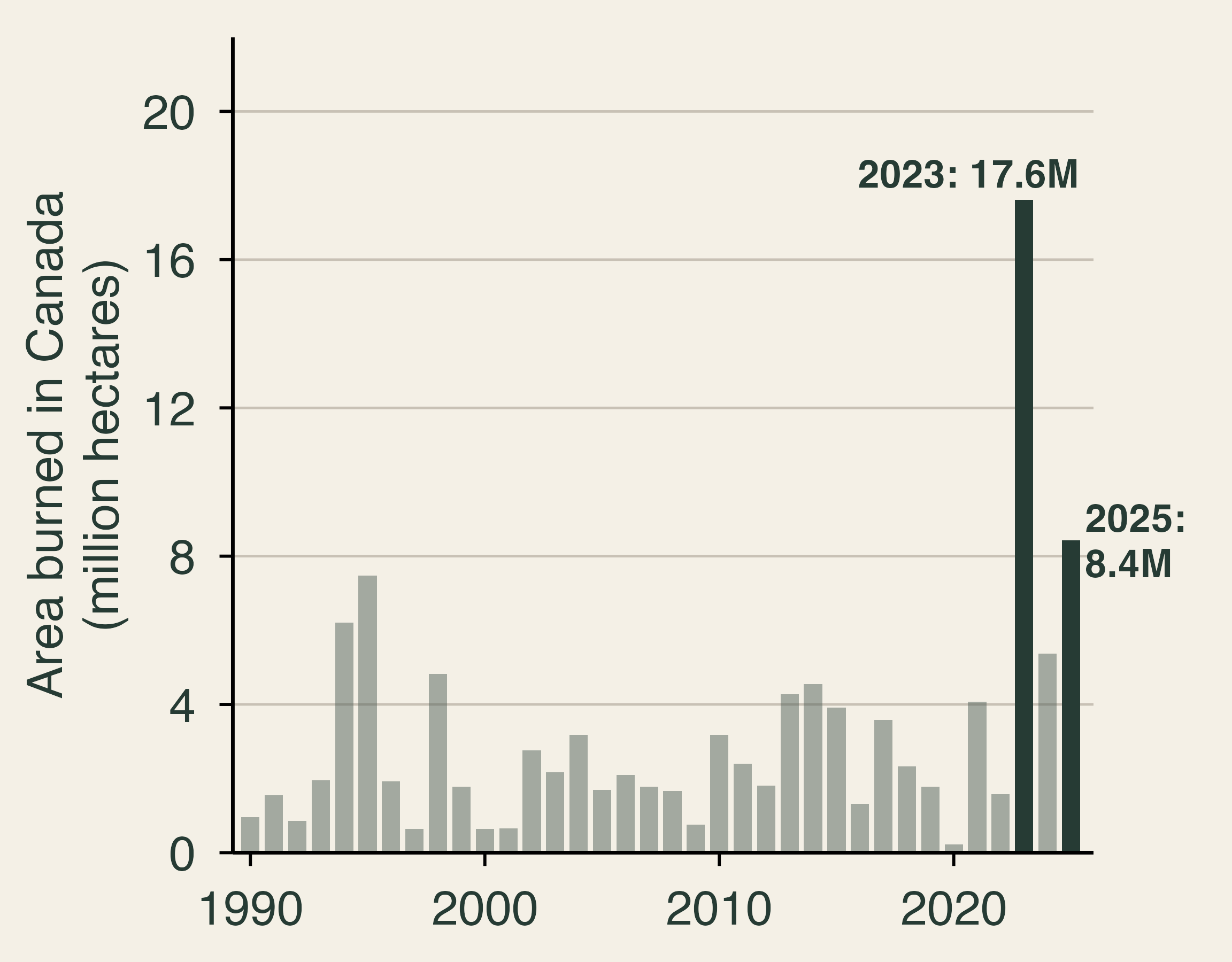
Canada’s 2023 fire season was the largest in its recorded history. Summing the totals that provincial and territorial agencies report to the National Forestry Database, about 17.6 million hectares burned, more than twice the largest earlier year in the database, 7.5 million hectares in 1995, and about seven times the 1990–2022 average of 2.4 million. The national record before 2023, set in 1989, was about 7.6 million hectares (Canadian Interagency Forest Fire Centre, 2024). Agency totals count everything inside fire perimeters, including unburned islands, lakes, and bare ground, so satellite mapping gives a smaller number: 15.0 million hectares, still more than twice the 1989 record measured the same way (Natural Resources Canada, 2024; Jain et al., 2024). A record 232,000 people from 200 communities were evacuated. Most of the burned area lay in remote boreal forest, so property losses were small relative to the area burned. The damage that traveled was smoke. The 2025 season, at about 8.4 million hectares, was the second largest in the series.

Area burned in Canada, 1990–2025, summed over the 12 provinces and territories that report to the National Forestry Database (Nunavut and Parks Canada are not in this table). Source: National Forestry Database, Canadian Council of Forest Ministers.

June 2023 in the East

On June 6–8, 2023, smoke from fires in Quebec drifted south over New York, Pennsylvania, and the mid-Atlantic. We built the figure below from the U.S. Environmental Protection Agency’s Air Quality System, averaging the 24-hour PM_2.5 readings across all monitors in each metro area. On June 7, the average monitor in the New York metro area recorded 153 micrograms per cubic meter (µg/m³), more than four times the EPA’s 24-hour standard of 35 µg/m³, and the highest single hourly reading was 412 µg/m³. Philadelphia (181 µg/m³) and Syracuse (182 µg/m³) were higher still. A second wave reached Chicago (130 µg/m³ on June 27) and Detroit (127 µg/m³ on June 28) and then drifted east again. For comparison, the median day of 2023 in these metro areas ran between 6 and 10 µg/m³. City officials reported an air quality index of 484 that afternoon, just short of the top of the scale at 500 (New York City Public Advocate, 2023). Before 2023, the city’s highest daily average on record was about 86 µg/m³, set in July 2002 (Joo et al., 2024).

Daily PM_2.5 in six eastern metro areas, late May to early July 2023. Each line averages the 24-hour readings of a metro area’s monitors, and the dashed line marks the EPA 24-hour standard. Source: U.S. EPA Air Quality System.

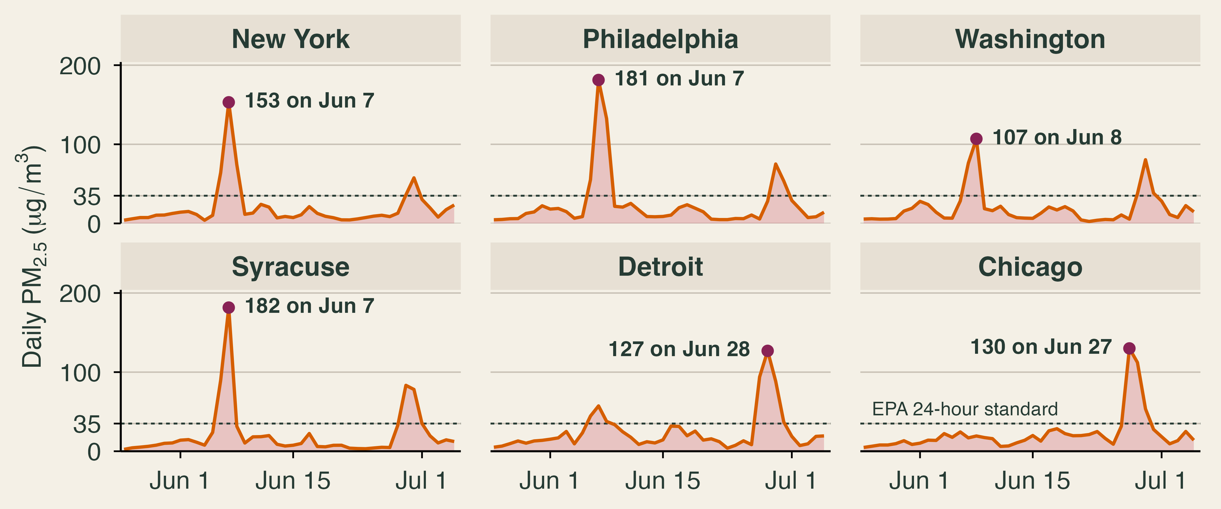
Two details of the data are worth knowing. First, Rochester’s main monitor stopped reporting complete days during the June 6–7 peak, so the figure uses Syracuse for upstate New York; EPA’s daily air quality index (AQI) for the Rochester metro area still rated both days “unhealthy.” Second, state agencies can flag smoke-affected readings as “exceptional events,” for reasons explained below. EPA’s files keep both versions, and we use the readings with the smoke left in, because that is the air people breathed.

Smoke and the Clean Air Act

Fine-particle pollution in the eastern United States fell sharply after 2000 as regulations under the Clean Air Act cut emissions from power plants, vehicles, and industry. The next figure counts the days each year on which PM_2.5 pushed a metro area’s AQI above 100, the level at which air becomes unhealthy for sensitive groups. We leave out July 4 and 5, when fireworks rather than fires cause short spikes. New York had 18 such days in 2000 and 23 in 2001, and between zero and two in every year from 2015 to 2022. Rochester never had more than three in a year from 2000 to 2022. Then the smoke arrived: six days in New York and eight in Rochester in 2023, and three and seven in 2025, another severe Canadian season.

Days per year on which PM_2.5 pushed the metro area’s AQI above 100, leaving out July 4 and 5. Orange bars mark 2023 and 2025, two severe Canadian fire seasons. Source: U.S. EPA AirData.

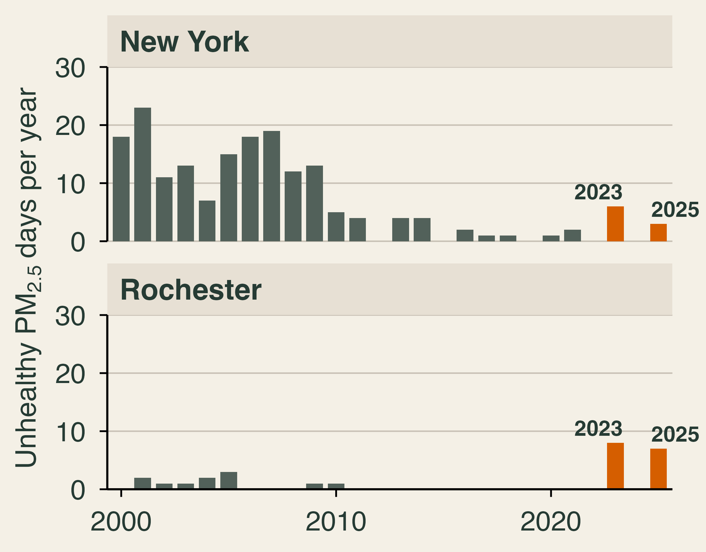
Burke et al. (2023) document the same reversal across the country, using data through 2022, before the Canadian smoke of 2023 reached the East. Wildfire smoke had a statistically significant influence on recent trends in annual average PM_2.5 in 35 of the 48 contiguous states. Since about 2016, smoke has erased about a quarter of the earlier gains in those states on average, roughly four years of progress, and more than half in many western states. Through 2022, many northeastern states showed no detectable influence. The 2023 and 2025 seasons in the figure above suggest that the East has now joined the West.

Smoke also sits outside the usual machinery of regulation. The Clean Air Act works by controlling sources, such as a power plant, a refinery, or a car, and a forest fire in Quebec has no permit to revise. Under EPA’s Exceptional Events Rule (U.S. EPA, 2016), states can ask EPA to set aside monitoring data affected by events such as wildfires when it decides whether an area meets the air quality standards. The rule is sensible for regulators, since New York cannot control a fire in another country, but it also means that no one is charged for the damage.

The health bill and the value of a statistical life

The health effects arrived within hours. In New York City, asthma-related emergency department visits rose from about 182 a day in comparison periods to 261 a day during the June 6–8 smoke wave, a 44% increase, while the city’s average PM_2.5 rose from 9.0 to 100.9 µg/m³ (Chen et al., 2023). In the rest of New York State, asthma visits on June 7 were 82% above their June 1–5 average, and they nearly tripled among people aged 10 to 29 (Meek et al., 2023). Across the country, the Centers for Disease Control and Prevention (CDC) found that asthma visits ran 17% above expected on the 19 smoke days between late April and early August 2023 (McArdle et al., 2023).

Deaths are harder to measure, because smoke rarely appears on a death certificate. Researchers instead combine estimates of exposure with studies that link PM_2.5 to the risk of dying. Zhang et al. (2025) estimate that smoke from the 2023 Canadian fires added 1.49 µg/m³ to annual average PM_2.5 in the United States. They attribute about 4,100 U.S. deaths (95% CI: 2,600 to 5,600) to short-term exposure on smoke days and about 33,000 (95% CI: 22,500 to 43,500) to the added long-term exposure. The two numbers come from different methods and should not be added. The gap between them shows how much the answer depends on the exposure-response relationship a study chooses. Looking at all wildfire smoke rather than one season, Qiu et al. (2025) estimate about 41,000 smoke-related deaths a year in the United States over 2011–2020 and project 71,420 a year by 2050 under a high-warming scenario (95% CI: 34,930 to 98,430).

U.S. deaths attributed to smoke from the 2023 Canadian wildfires, by two methods that should not be added. Error bars show 95% confidence intervals. Source: Zhang et al. (2025).

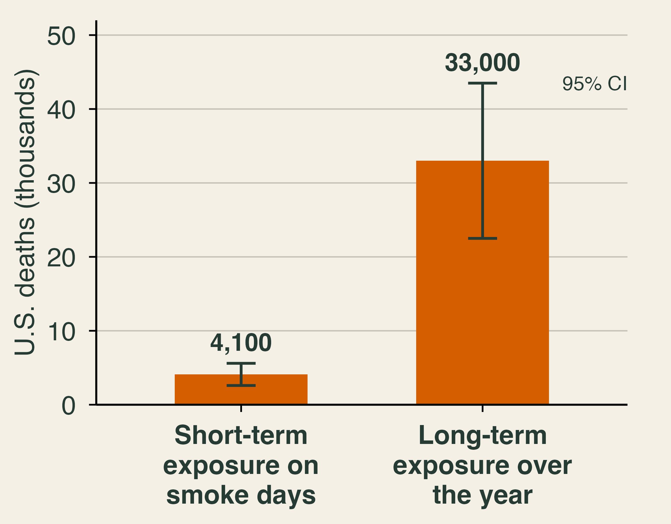
To compare deaths with dollars of lost work and medical bills, economists use the value of a statistical life (VSL). The VSL is not the value of any particular person. It summarizes how much people are willing to pay for small reductions in their risk of death. Suppose each of 100,000 people would pay $142 to reduce their risk of dying this year by 1 in 100,000. Together they would pay $14.2 million, and on average the reduction saves one life among them, though no one knows whose. That is a VSL of $14.2 million. Agencies estimate the VSL from the extra wages workers demand for riskier jobs and from surveys, the revealed and stated preference methods of Lecture 7. The U.S. Department of Transportation currently uses $14.2 million for analyses with a 2025 base year (U.S. Department of Transportation, 2026). EPA recommends a central value of $7.4 million in 2006 dollars, updated for inflation and income growth to the year of the analysis (U.S. EPA, 2026); Qiu et al. (2025) use EPA’s value of $10.95 million in 2019 dollars.

\text{Mortality damage} = \text{Deaths} \times \text{VSL}.

Applied to the short-term estimate for 2023, the mortality damage is 4{,}100 \times \$14.2 \text{ million} \approx \$58 billion. The long-term estimate implies nearly half a trillion dollars, although deaths from long-term exposure arrive over several years and should be discounted. Either way, the deaths dwarf the direct firefighting costs of a typical U.S. year, about $3 billion in federal suppression spending (Section 4).

Three cautions apply. The VSL measures willingness to pay for small changes in risk across many people, not the worth of a named individual. Willingness to pay rises with income, yet U.S. agencies apply one value to everyone, a choice made on equity grounds. And smoke deaths are concentrated among older adults and people with heart and lung disease, which raises the question of whether a year of life lost should count the same at every age.

Smoke and paychecks

Smoke also hurts people who never see a doctor. Borgschulte, Molitor, and Zou (2024) combine satellite data on smoke plumes with county labor-market data and find that each additional day of smoke exposure reduces quarterly earnings by about 0.1%. Lost jobs and people leaving the labor force explain only 13% of the decline. Most of it comes from lower earnings among people who keep working, through fewer hours, sick days, time spent caring for others, or lower productivity. Summed over the smoke days Americans experienced, the working-paper version of the study puts the losses at nearly 2% of U.S. labor income, about $125 billion a year in 2018 dollars on average over 2007–2019 (Borgschulte, Molitor, and Zou, 2022). That period ends before the 2023 season.

Why might lost pay exceed the medical bills? Hospital visits are rare, while a smoke day touches millions of workers at once, and small losses spread over a large workforce add up. In the authors’ comparison, the lost earnings per unit of smoke exceed the mortality costs they compute from the medical literature, although that ranking depends on which mortality estimate and VSL one uses. Lost earnings never appear in a fire’s damage tally, which is one reason smoke is easy to underestimate.

Defensive spending and who can afford it

People do not sit still while smoke rolls in. They close windows, run air purifiers, wear N95 masks, cancel outdoor plans, and stay home. Kahn (pp. 63–66) stresses that people are not passive victims: forecasts warn of smoke days ahead, cheap monitors measure indoor air, and markets supply purifiers that cost about a hundred dollars. Burke et al. (2022) document these responses across the United States. On days with more smoke, online searches for air filters, air purifiers, smoke masks, and air-quality monitors all rise. On days with smoke PM_2.5 above 50 µg/m³, the share of people who stay home all day rises by about three percentage points, a modest change given the health risk. The responses differ by income: searches for protective products show no detectable rise in roughly the poorest third of counties, while people in wealthier counties stay home more.

Spending to protect yourself from pollution is called defensive spending or averting behavior. It links smoke to the valuation methods of Lecture 7. If a household spends $250 on a purifier and masks to get through a smoke episode, it must value the protection at no less than $250, and the purifier does not remove all of the harm. So defensive spending gives a lower bound on willingness to pay to avoid smoke. A full accounting adds the remaining health and work losses and the discomfort that no one pays to avoid.

One smoke episode, two households. Defensive spending is visible in market data; the remaining harm is not. Classroom numbers.

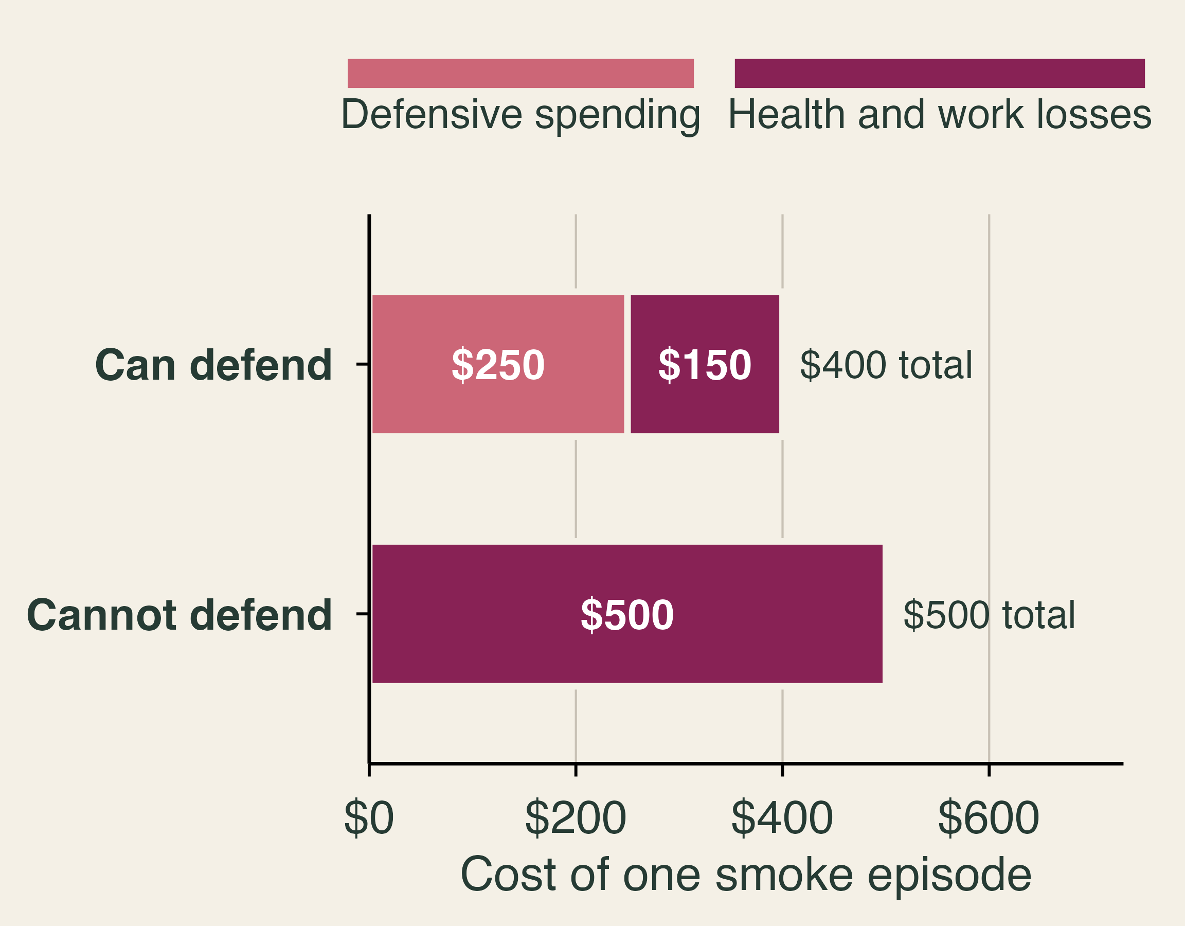
The classroom numbers above make the equity point. The household that can defend spends $250 and still loses $150 in health and work, for a total of $400. The household that cannot defend, because it rents an apartment without central air, works outdoors, or cannot spare $250, spends nothing and loses $500. A researcher who measured smoke’s cost by purifier sales would record $250 of damage for the first household and none for the second. Kahn (p. 186) notes that richer people are willing to pay more to be safe, and defense is one way they buy safety. This pattern is an environmental justice concern: the same smoke imposes larger health costs on those least able to defend against it.

A transboundary externality

The 2023 smoke is a textbook externality with one unusual feature: it crosses a national border. Let R be the amount of smoke reduction that Canada undertakes, through fuel management and fire suppression near forests whose smoke reaches populated areas. Each unit of R costs Canada more than the last, so the marginal cost rises. The benefits fall as R grows. Canada’s government weighs the benefits to Canadians, including Canadian cities downwind, and chooses R_C, where its marginal benefit equals marginal cost. The benefits to Americans in New York and Chicago do not enter that decision. The efficient level for the two countries together, R^*, sets the combined marginal benefit equal to marginal cost, and the shaded triangle is the value lost at R_C.

Smoke reduction in Canada with a benefit to the United States. Canada’s choice R_C falls short of the joint optimum R*. Stylized figure.

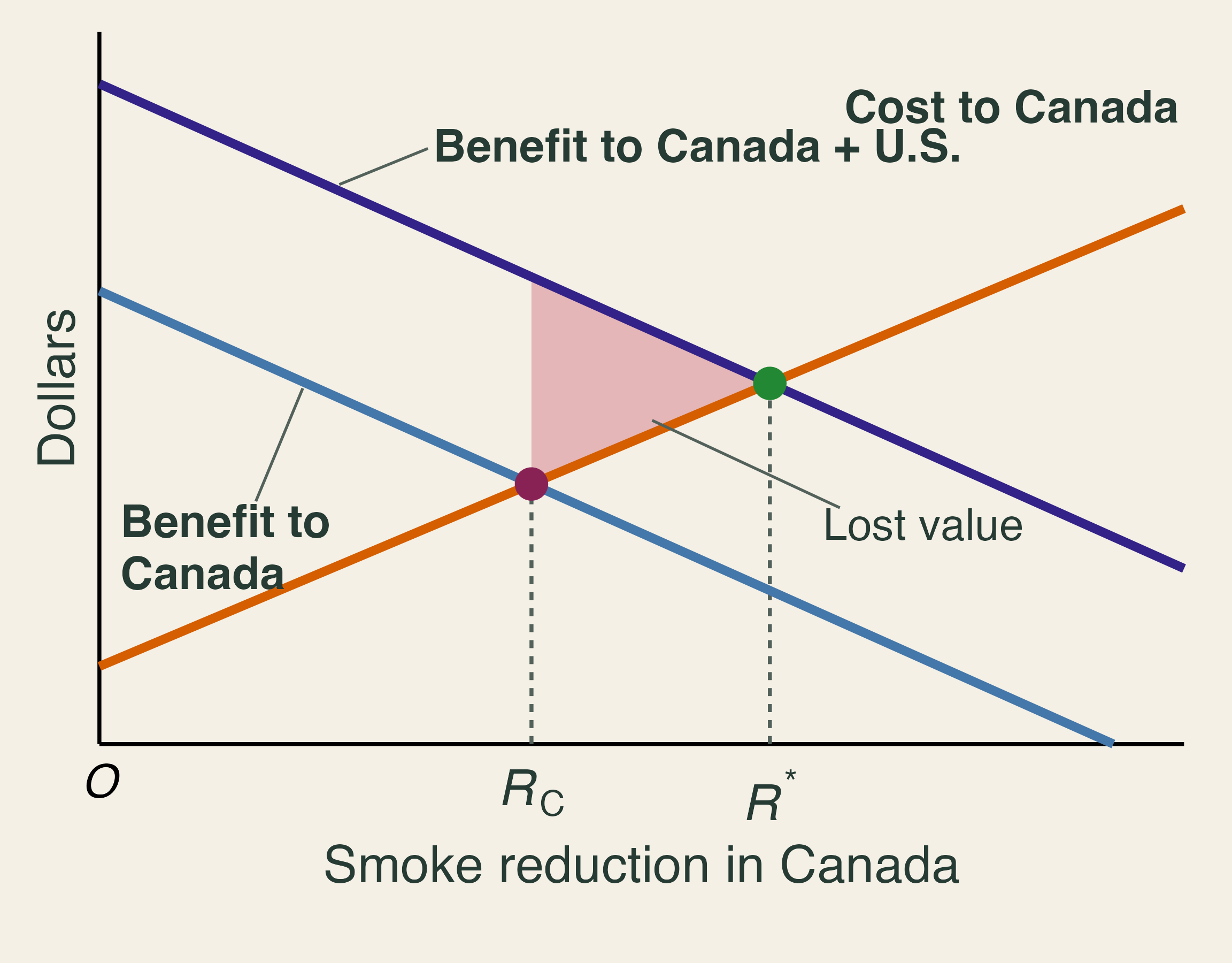
Why don’t the two countries simply bargain? The Coase theorem says that, with clear property rights and low transaction costs, the parties will reach the efficient outcome whoever holds the rights. Kahn (p. 114) applies the theorem to smoke from public forests: if downwind residents had a right to clean air, they could sue the landowner, and if the landowner had the right, the residents would have an incentive to pay for brush clearing. Across a border, both routes are hard. Millions of people are affected, no court enforces a cross-border right to clean air, and each country can free ride on the other’s efforts. The externality also runs both ways, since smoke from fires in the western United States regularly drifts into Canada, which gives both countries a reason to cooperate. Some cooperation already exists. Under a reciprocal firefighting arrangement in place since 1982, the two countries lend each other crews and equipment, and in 2023 the United States was Canada’s largest source of outside help, with about 2,450 personnel (Canadian Interagency Forest Fire Centre, 2024). That cooperation targets flames rather than smoke. The 1991 Canada–United States Air Quality Agreement, written for acid rain and later extended to ozone, does not deal with wildfire smoke. A 2024 joint review by the two countries’ environment agencies noted that recent wildfire smoke had caused harm along the length of the border and recommended updating the agreement (Environment and Climate Change Canada and U.S. EPA, 2024). Reciprocity in firefighting shows that a deal on smoke is possible, even if none exists yet.

Two further points keep the graph honest. First, much of Canada’s burned area lies in remote boreal forest where suppression is costly, often ineffective against the largest fires, and not always desirable, because fire is part of how these forests renew. In Quebec, for example, the provincial fire agency SOPFEU fights fires across an intensive protection zone in the populated south, while north of the 51st parallel it “intervenes only on fires that threaten communities or strategic infrastructure” (SOPFEU, 2026). Ontario likewise monitors some fires that are far from communities, homes, and timber (Government of Ontario, 2019). In 2023, about 4.3 million hectares burned under a monitored response, and 147 fires burned 3.4 million hectares in Quebec’s northern zone alone (Canadian Interagency Forest Fire Centre, 2024). The efficient R^* may therefore be modest, and much of the gain may come from protecting communities and from the United States adapting at home. Second, climate change raises the hazard on both sides of the border, so cutting emissions, the mitigation of Section 1, is the long-run complement to any cooperation over smoke. Mitigation is a global public good, which makes it even harder to provide than cooperation between two neighbors.

3. Deciding under risk

Textbook reading. TL Chapter 12. Kahn, pp. 11, 31–32, 92–94, 119, and 193.

Expected value and a fuel-treatment project

Suppose a house has a 2% annual chance of a fire that causes $100,000 in damage (Kahn, p. 119). Its expected annual damage is 0.02 \times \$100{,}000 = \$2{,}000. No year ever produces a $2,000 loss. In 98 of 100 years the owner loses nothing, and in two years the owner loses $100,000. Expected value is an average across possible years, not a forecast of next year’s bill.

Public projects can be evaluated the same way. Let P(x_i) be the probability of outcome x_i and NB(x_i) its net benefit. The expected net benefit is

E[NB] = \sum_i P(x_i) \times NB(x_i).

Consider a county that can spend $7 million on thinning and prescribed burns. The numbers below are classroom values, and each net benefit already subtracts the cost.

Fire seasons	Net benefit	Probability	Probability × net benefit
Mild	$5 million	0.27	$1.35 million
Average	$10 million	0.49	$4.90 million
Severe	$20 million	0.23	$4.60 million
Prescribed burn escapes	−$100 million	0.01	−$1.00 million

The probabilities sum to one, as they must when the list of outcomes is complete. Adding the last column gives E[NB] = \$9.85 million, so a cost-benefit test says to proceed. Notice how little the worst row matters: a $100 million loss moves the answer by only $1 million.

Expected net benefit of the fuel-treatment project, built up one outcome at a time. Classroom numbers.

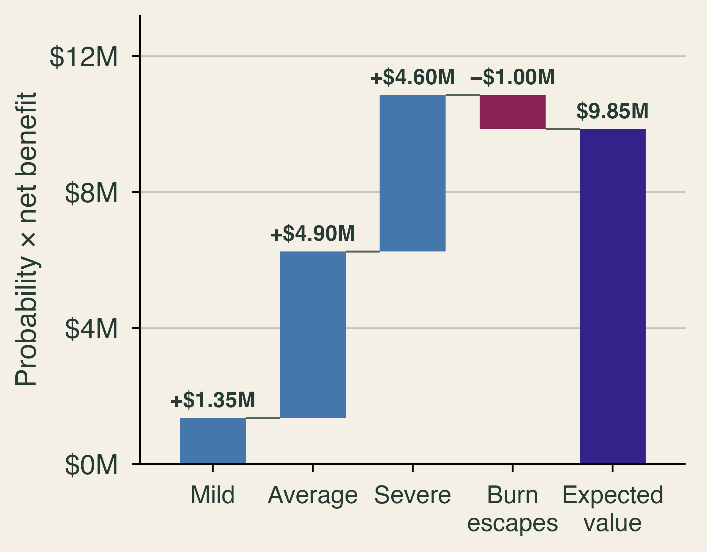
When the 1% branch happens

That last row is not far-fetched. The Forest Service reports that 99.84% of its prescribed fires go according to plan, and that even a very small share of escapes can have severe consequences (U.S. Forest Service, 2022). In 2022, two escaped burns in New Mexico, the Hermit’s Peak and Calf Canyon fires, merged into a fire of about 341,000 acres, and Congress set aside $3.95 billion to compensate victims. The neighbors bore the loss first, and federal taxpayers then funded the compensation. Prescribed fire also has a cost in smoke. Schollaert et al. (2024) find that moderate burning lowers wildfire smoke exposure in a California landscape, but the gain levels off as burning grows because treatment smoke adds up. Burns add some smoke now to prevent more smoke later.

Risk aversion

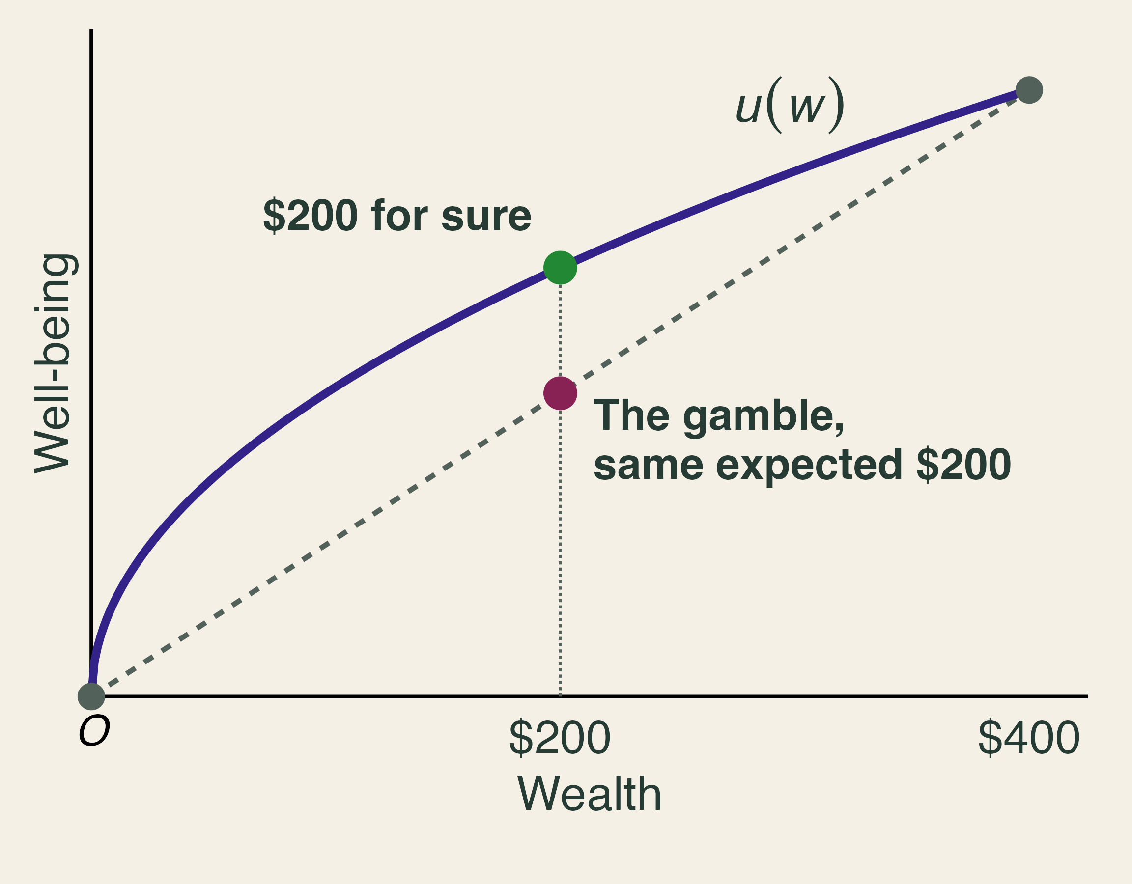
Expected value treats a sure $200 and a coin flip for $400 or nothing as equal (Kahn, p. 32). Most people take the sure thing, and economists call this risk aversion. The reason is diminishing marginal utility: each extra dollar adds less well-being than the one before, so losing $200 hurts more than gaining $200 helps. On a graph of well-being against wealth, the curve bends. The sure $200 lies on the curve, while the gamble lies on the straight line below it at the same expected wealth.

Risk aversion. With a concave well-being curve, a sure $200 beats a gamble with the same expected value.

A worked example shows how large the effect can be when the gamble is your home. Suppose a household’s wealth is a $400,000 house, the house has a 2% annual chance of burning down, and well-being is the square root of wealth, U(W) = \sqrt{W}. Expected wealth is 0.98 \times \$400{,}000 = \$392{,}000. Expected well-being is

E[U] = 0.98 \times \sqrt{400{,}000} + 0.02 \times \sqrt{0} \approx 619.8.

The certainty equivalent is the sure wealth that gives the same well-being: 619.8^2 \approx \$384{,}160. The household would therefore pay up to \$400{,}000 - \$384{,}160 = \$15{,}840 a year to remove the risk entirely, nearly twice its expected loss of $8,000. The difference, $7,840, is the risk premium. Insurers can charge more than expected losses and still find buyers because of this gap.

Risk versus uncertainty

Under risk, we can list the outcomes and trust the probabilities. Under uncertainty, we cannot. Fire records from the past may be a poor guide when climate, fuels, and development are all changing. Kahn (p. 11) puts it plainly: “we know that we do not know the probabilities” of disasters such as wildfires. Even professionals disagree, as Boomhower et al. (2024) document in the “striking variation” across insurers’ classifications of wildfire risk. Canada’s 2023 season, discussed in Section 2, burned more than twice the area of any earlier year on record, which is the kind of event a backward-looking model would assign almost no probability.

Under uncertainty, no single formula replaces E[NB]. Planners use a margin of safety, test a project against a worst plausible case, or prefer actions that perform reasonably well across many scenarios. Kahn offers a counterweight: protection has a rising marginal cost, one cannot “triple bubble-wrap” a home (p. 193), and money spent on one risk is unavailable for another, so we should look for the most “bang per buck” (p. 93).

Do building codes work?

Baylis and Boomhower (2026) offer some of the best evidence on hardening. Using U.S. homes exposed to wildfires since 2000, they compare homes that faced identical fire exposure but were built in different years and under different code rules. In their sample, 39% of exposed homes were destroyed. A California home built in 2008 or later was about 13 percentage points less likely to be destroyed than a 1990 home in the same fire, a 34% reduction relative to that average. Earlier working-paper versions of the study reported larger effects; we use the published estimates.

What 13 percentage points means for 100 exposed homes. The 39 lost is the sample average, not the rate for a 1990 home. Source: Baylis and Boomhower (2026).

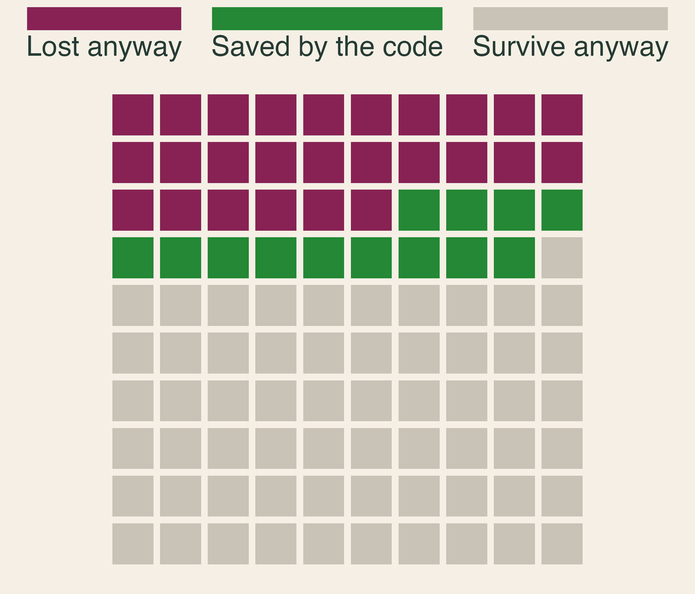
Do codes pass a cost-benefit test? It depends on when the work is done. Baylis and Boomhower estimate that building a new home to code costs about $15,660, which pays off when the annual chance of a damaging fire exceeds 0.34%. A full retrofit of an older home costs about $62,760 and needs 1.35%. Targeted codes raise welfare by about 20% relative to no policy, partly because hazard and neighbor density are visible in advance. Because codes for new homes are far cheaper than retrofits, where new homes get built matters.

My roof protects your house

The benefits of a code spill over. A pre-code neighbor within 10 meters raises a home’s chance of destruction by about 1.7 percentage points, or 4.4%, because fire spreads from structure to structure (Baylis and Boomhower, 2026). Hardening therefore has a positive externality. The owner compares private benefit with cost and stops at h_P, short of the efficient level h^* that also counts the neighbors. The shaded triangle is the value lost because the neighbors’ benefit does not enter the owner’s decision.

Hardening with a positive externality. The private choice is below the efficient level, and the shaded area is lost value.

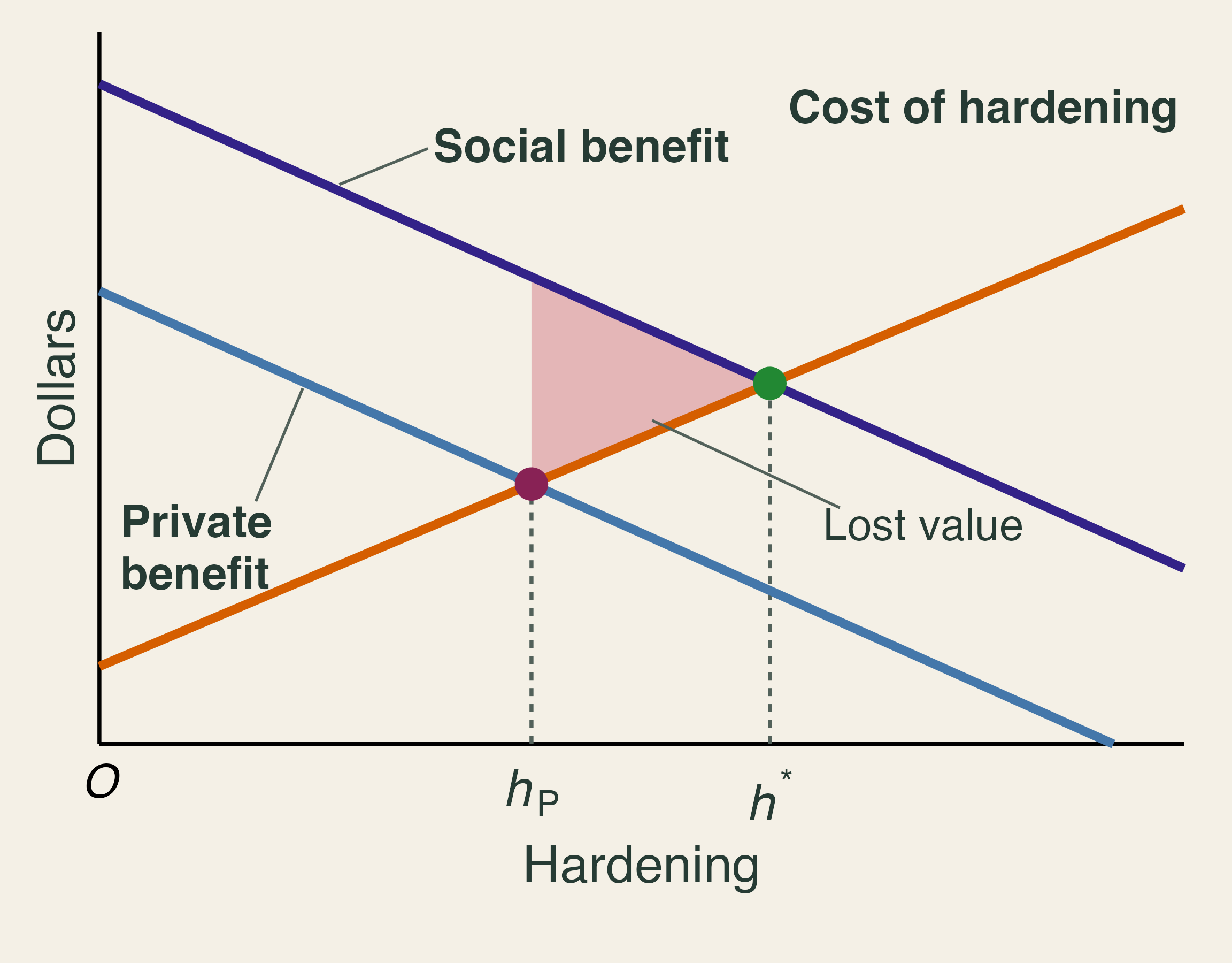
A numerical version makes the gap concrete. Suppose a $10,000 retrofit avoids $2,000 a year of expected damage to the owner’s home and $500 a year to the neighbors, for five years, at a 4% discount rate. The present value of $1 a year for T years at rate r is the annuity factor,

AF = \frac{1 - (1 + r)^{-T}}{r} = \frac{1 - 1.04^{-5}}{0.04} \approx 4.4518.

For the owner alone, the benefit is worth \$2{,}000 \times 4.4518 = \$8{,}904, a net loss of $1,096. Counting the neighbors, it is worth \$2{,}500 \times 4.4518 = \$11{,}130, a net gain of $1,130. A grant of at least $1,096 would change the owner’s choice. A mandate could achieve the same result without public money, but it would also force hardening on owners for whom it does not pay, which is the trade-off Baylis and Boomhower weigh. Why don’t neighbors simply pay each other, as the Coase theorem suggests? Many households share each spillover, each hopes the others will pay, and work on a roof or vent is hard to verify. Homeowners associations can partly internalize the spillover (Kahn, p. 144).

4. Sharing the risk

Textbook reading. TL Chapter 12. Kahn, pp. 7, 79, 84, 87, 115–129, and 141–148.

A household’s choice

For most families, a home is the largest asset they will ever own. Kahn calls this holding a “one place-based egg” (pp. 7, 84). Suppose a house has a 2% annual chance of a total loss with a $400,000 rebuilding cost, so the expected annual loss is $8,000. Consider three options, using classroom numbers:

Option	Premium	You pay if it burns	Expected yearly cost	Insurer’s expected claim
A: No insurance	$0	$400,000	$8,000	$0
B: Partial, subsidized	$5,000	$100,000	$7,000	$6,000
C: Full, risk-based	$9,500	$2,500	$9,550	$7,950

The expected yearly cost adds the premium to the expected out-of-pocket loss. For option C, that is \$9{,}500 + 0.02 \times \$2{,}500 = \$9{,}550. The insurer’s expected claim is 2% of what it pays in a fire: 0.02 \times \$397{,}500 = \$7{,}950 for C and 0.02 \times \$300{,}000 = \$6{,}000 for B.

Option C costs the most on average and removes the ruinous year, which is what a risk-averse household is buying. The $1,550 gap between C’s premium and its expected claim, called the loading, pays for administration, capital, and reinsurance. Option B is cheap for a different reason: its premium is below its expected claim, so someone else covers the difference. With the square-root utility from Section 3, the certainty equivalents are about $384,160 for A, $390,450 for C, and $392,860 for B. The household prefers C to A even though C costs $1,550 more a year on average, and it prefers B to both because B carries a subsidy. A subsidy that makes partial coverage the best choice is a theme we will meet again.

Pooling and correlated losses

Insurance works by pooling losses that do not happen together. If 1,000 homes each face an independent 2% chance of fire, the number of fires in a year follows a binomial distribution with a mean of 20 and a standard deviation of \sqrt{1{,}000 \times 0.02 \times 0.98} \approx 4.4. In 99% of years, between 10 and 32 homes burn, so the insurer can predict its claims within a narrow band. This is the law of large numbers at work.

Wildfire breaks that assumption, because a fire jumps from roof to roof. Kahn (p. 116) asks us to imagine 1,000 homes in Pacific Palisades, each insured for $1 million. Add a 2% annual chance of fire, and expected claims are $20 million either way. If fires strike independently, claims land between $10 million and $32 million in 99% of years. If all the homes burn together, claims are zero in 98% of years and $1 billion in the other 2%.

Same expected claims, different risk for the insurer. Based on Kahn (2026, p. 116), with a 2% fire chance added.

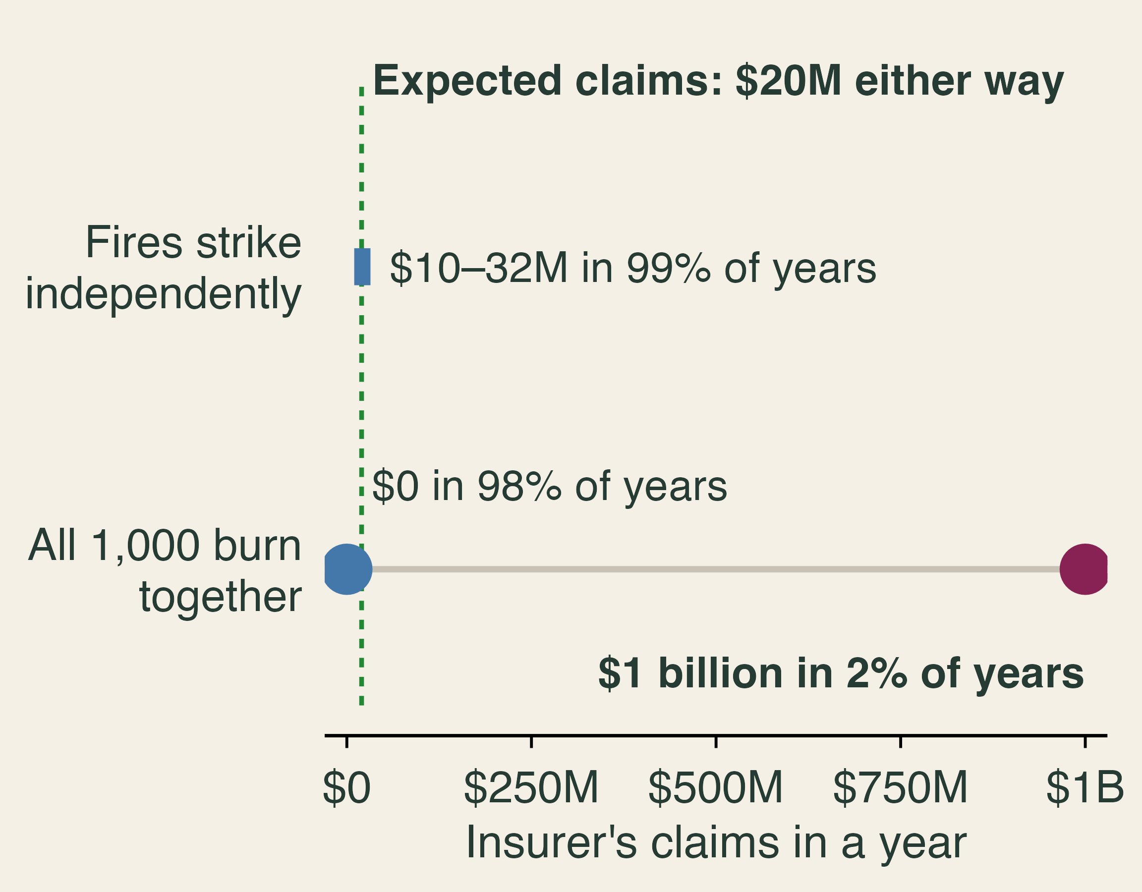
The expected claim cannot tell us how much money must be on hand after a severe year. An insurer facing correlated losses must hold capital, spread policies across regions, or buy reinsurance, which is insurance for insurers. These costs rise with the tail, not with the average, so premiums in fire country must cover more than expected losses.

Premiums and price ceilings

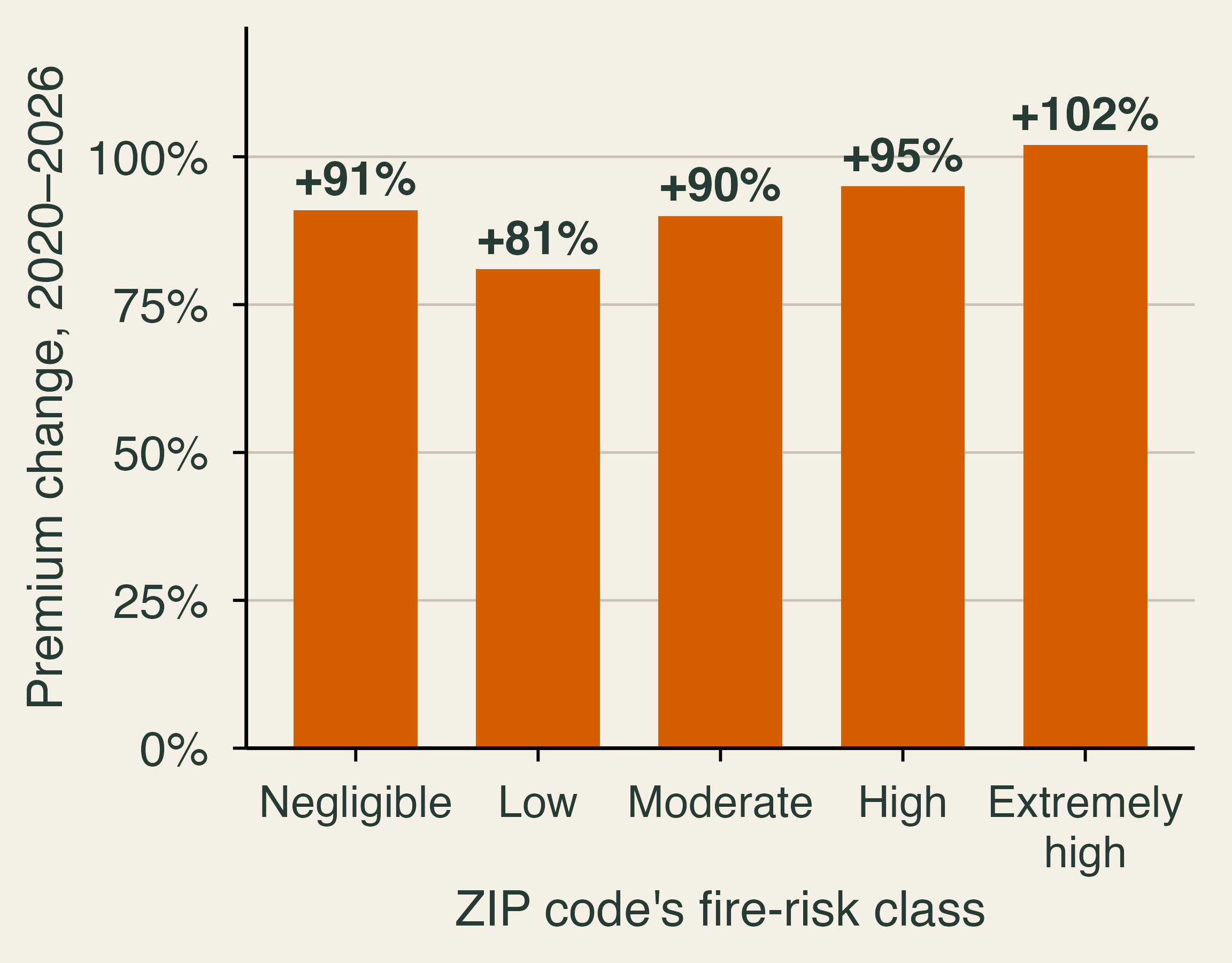
Premiums have responded. Using over 74 million premiums from 2014 to 2024 inferred from mortgage escrow payments, Keys and Mulder (2024) document a doubling in the pass-through of disaster risk into premiums, and show that higher premiums cut home price growth by over $40,000 in the most exposed ZIP codes. They link part of the rise to the repricing of catastrophe risk in global reinsurance markets. In California, Nguyen et al. (2026) find that the average premium rose 84% between 2020 and 2026, or 45% after inflation. The increase was similar across fire-risk classes, from 81% in low-risk ZIP codes to 102% in extremely high-risk ones. When premiums rise almost equally everywhere, prices are not sorting risk. California’s premiums have also stayed near 85% of the rest of the country’s even as wildfire losses mounted, which the authors suggest may reflect regulation.

Nominal change in average California homeowners premiums, 2020–2026, by ZIP code fire-risk class. Source: Nguyen et al. (2026).

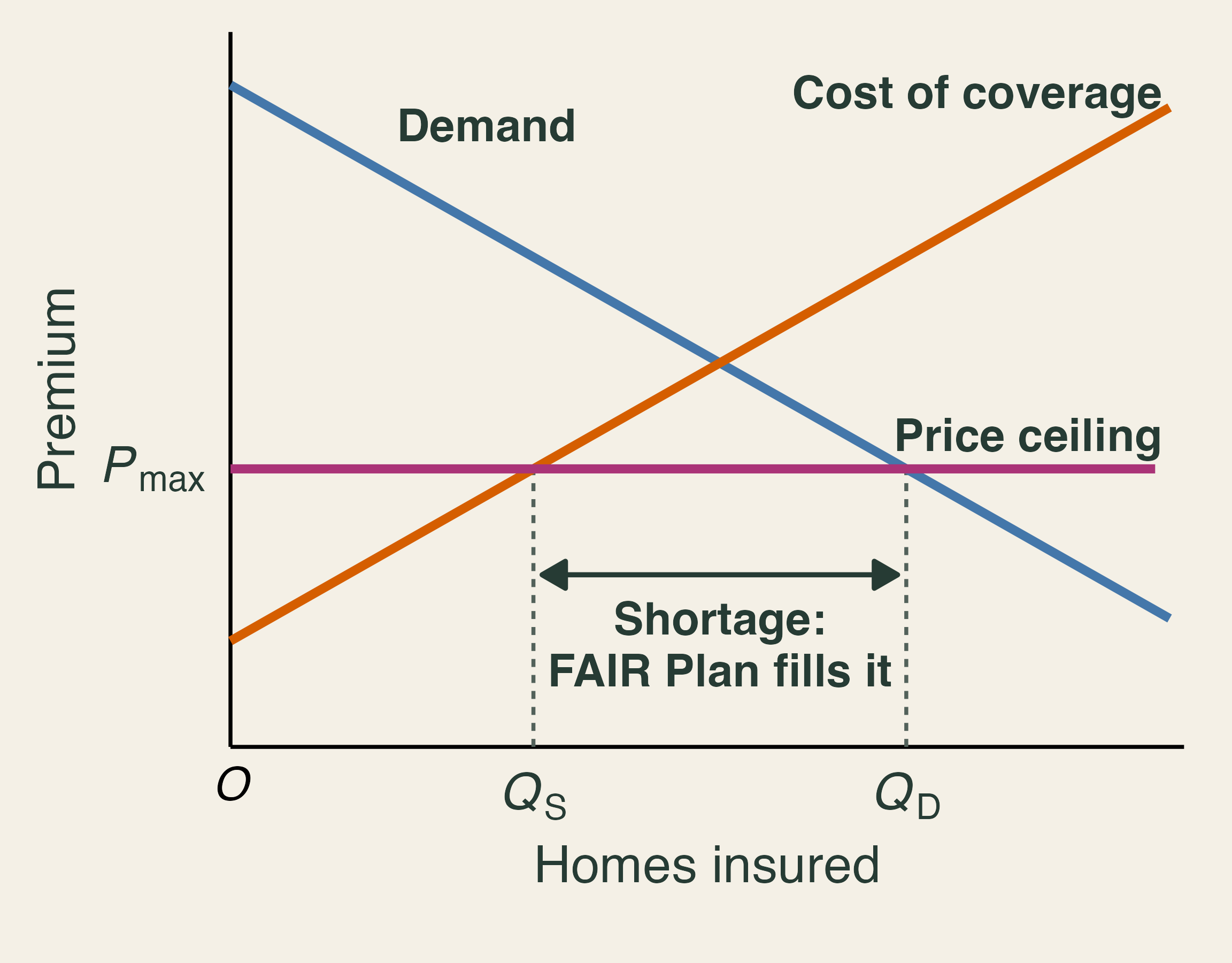
Under Proposition 103, passed in 1988, insurers need prior approval to raise rates, and approved rates long rested on past losses (Kahn, pp. 120, 143). Kahn argues that this acts as a price ceiling. When the allowed premium P_{max} falls below the price at which supply equals demand, insurers offer only Q_S policies while households want Q_D. Econ 101 predicts a shortage of Q_D - Q_S, and in insurance the shortage shows up as non-renewals, firms that stop writing new policies, and growth in the state’s insurer of last resort.

A binding price ceiling in the market for home insurance.

Regulation also serves a purpose: voters adopted Proposition 103 after large rate increases, and it can protect consumers from excessive rates. In December 2024, California began allowing catastrophe models and reinsurance costs in rate-making, and required insurers using them to write more policies in distressed areas. Nguyen et al. caution that solving availability in this way creates new affordability pressure, especially in high-risk areas.

The FAIR Plan and economic incidence

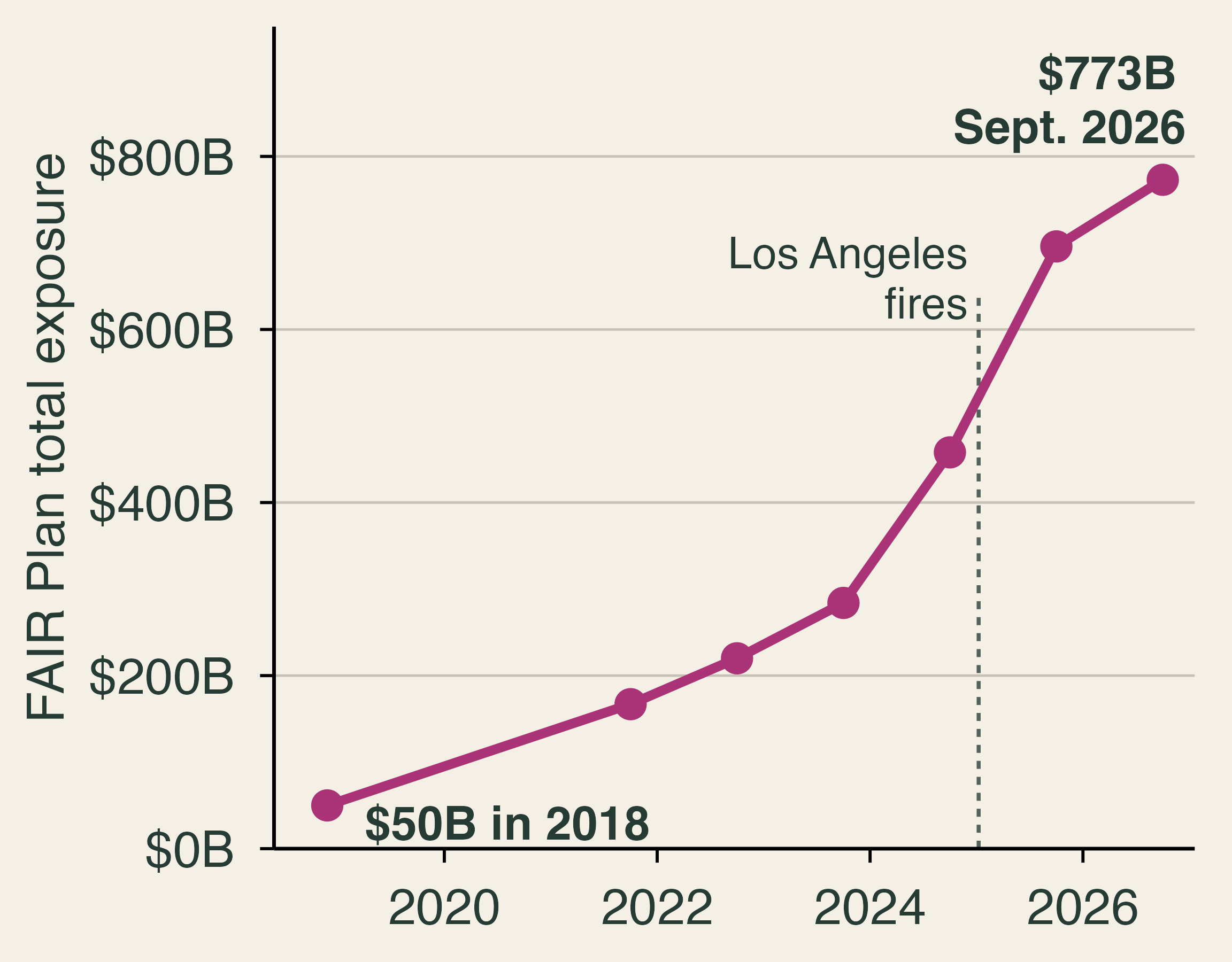
The California FAIR Plan, created in 1968, is an association of all licensed property insurers that sells basic coverage to owners who cannot find it elsewhere. Its total exposure, the sum of its policy limits, rose from $50 billion in 2018 to $773 billion in September 2026, and it now covers about 5% of the state’s single-family homes, up from about 2% in December 2020. Wallace (2026) writes that it “was never designed to serve as California’s primary wildfire insurer.” Nguyen et al. also find faster recent growth in low- and moderate-risk areas, which suggests a shortage of private coverage rather than high risk alone. The plan covers only basic property perils, so many customers buy a second, supplemental policy.

California FAIR Plan total exposure, the sum of policy limits. The 2021–2023 points are backed out of reported percentage changes. Sources: California FAIR Plan; Wallace (2026).

Who pays when the plan runs short? Kahn (p. 119) offers a simple illustration: a homeowner pays $1,000 for a policy with a 2% chance of a $100,000 claim, so the expected cost of $2,000 exceeds the premium and the owner receives a $1,000 subsidy. By statute, FAIR Plan rates must be actuarially sound, so whether a given policy is subsidized is an empirical question. Kahn also writes that taxpayers cover the deficit. The mechanism after the Los Angeles fires was more specific: in February 2025, the state approved a $1 billion assessment on member insurers, half of which they may recover through a temporary fee on policyholders (California Department of Insurance, 2025). Who is billed and who finally pays are different questions. The first is statutory incidence, which falls on insurers. The second is economic incidence, which can reach policyholders across the state, including low-risk ones, and insurers’ owners. Nguyen et al. describe the resulting cross-subsidy as an implicit tax on lower-risk policyholders.

Adverse selection

Adverse selection arises when those who buy at a given price are riskier than average, usually because buyers know more about their risk than the seller does or because the seller is not allowed to price what it knows. A classroom example shows the mechanism. Suppose half of the homes in a town have an expected claim of $1,000 a year and half have $5,000. If an insurer must charge everyone one price, the break-even price is the average, $3,000.

Adverse selection with one price for two kinds of homes. Classroom numbers.

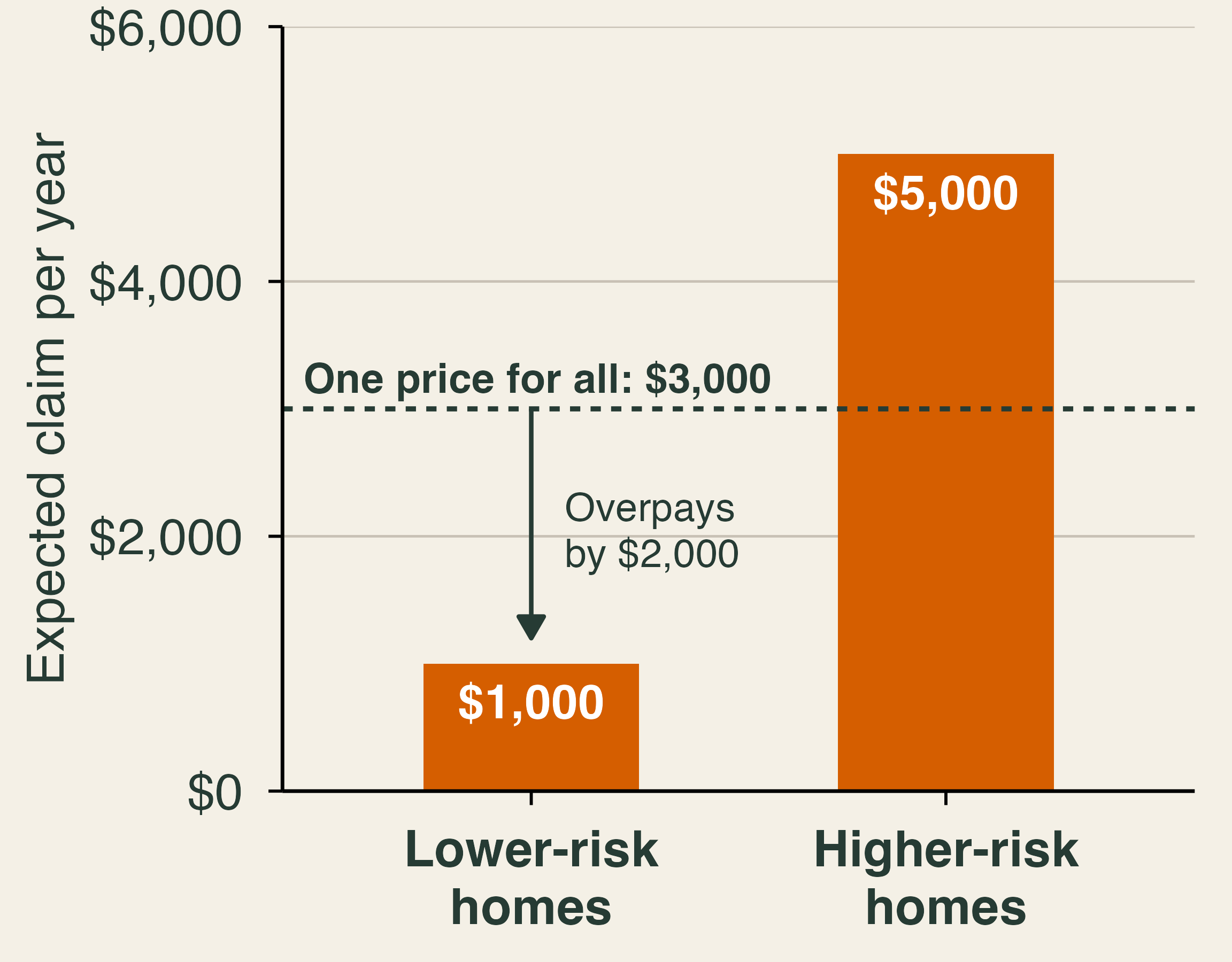
Lower-risk owners now pay $3,000 for $1,000 of expected protection. Even a risk-averse owner may refuse that deal, for instance by choosing a high deductible, moving to a cheaper insurer, or, without a mortgage, dropping coverage. If the lower-risk owners leave, the remaining pool expects $5,000 per home, and the price must rise to $5,000. In extreme cases the market unravels until only the riskiest buyers remain. Mortgage requirements slow this process, since most borrowers must keep coverage.

The same logic runs in reverse when insurers know more than one another. Boomhower et al. (2024) combine parcel-level wildfire risk data with regulatory filings for six large California insurers. Suppose one firm prices each parcel and another prices broad groups. Safer homes in each group get a better offer from the first firm, so the second firm is left with the riskier ones. Winning a customer becomes bad news, a winner’s curse, and firms with coarser models charge relatively high prices in high-risk segments or choose not to serve them. Kahn (p. 141) calls identifying the safer properties “cream skimming.” Either way, the riskiest homes end up concentrated in the FAIR Plan. Better risk models can improve incentives and still reduce participation in the market.

Moral hazard and free firefighting

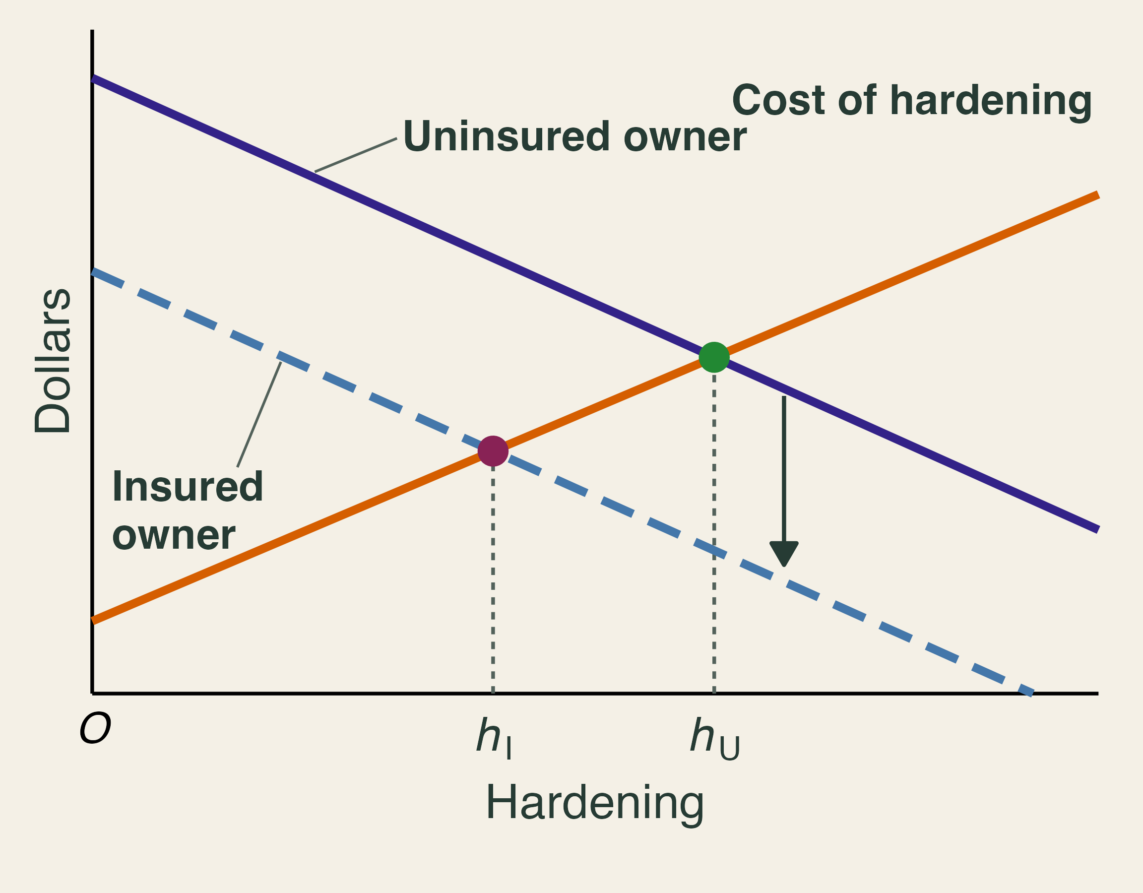
Moral hazard occurs when coverage changes behavior because the insured no longer bears the full cost. Kahn’s rule is that investors should not flip “one-sided coins” that keep the gains and pass along the losses (p. 87). If an insurer cannot see whether an owner has hardened a home, the owner’s private return to hardening falls, because the insurer collects much of the saving. In the graph, the insured owner’s marginal benefit curve lies below the uninsured owner’s, so the insured owner hardens less (h_I < h_U). The curve does not fall to zero, since insured owners still avoid disruption, deductibles, and uninsured losses.

Moral hazard in hardening. Insurance lowers the owner’s private return to hardening.

Pricing can reverse this if the action can be verified. Consider Kahn’s example (p. 142): a $5,000 premium for $400,000 in coverage. At a 2% fire risk, the insurer expects to pay $8,000 and loses $3,000. If the owner’s actions cut the risk to 1%, the expected payout falls to $4,000 and the insurer gains $1,000. There is now room to share the saving through a discount, and California’s Safer from Wildfires program lists steps that earn one. A home’s risk also depends on the street, though, so a discount for one owner can only go so far (Kahn, p. 134).

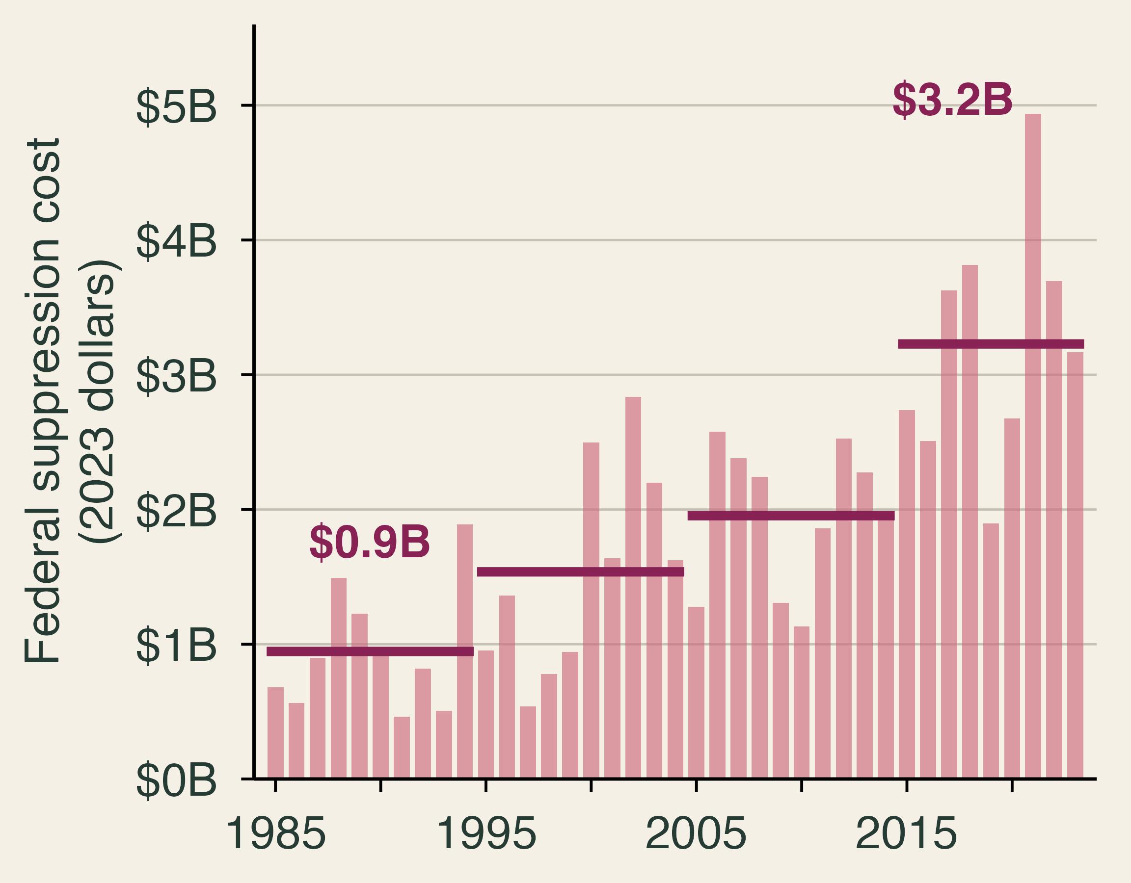
One form of wildfire protection is not called insurance at all. Governments fight fires for free. Real federal suppression spending rose from about $0.9 billion a year in 1985–94 to about $3.2 billion in 2015–23, a factor of 3.4. Baylis and Boomhower (2023) measure how nearby homes raise firefighting costs and find that the expected present value of this protection can exceed 20% of a home’s value. It rises with fire hazard and falls steeply with development density, so the largest implicit subsidies go to a small number of homes in risky, sparsely built places. Like cheap insurance, free protection weakens the price signal about where to build.

Federal wildfire suppression costs in 2023 dollars. Lines show period averages. Source: National Interagency Fire Center, deflated with the CPI.

5. Underinsurance, behavior, and recovery

Textbook reading. Kahn, pp. 40, 44–45, 73–76, 86–89, 123–124, and 200–201.

Too little coverage

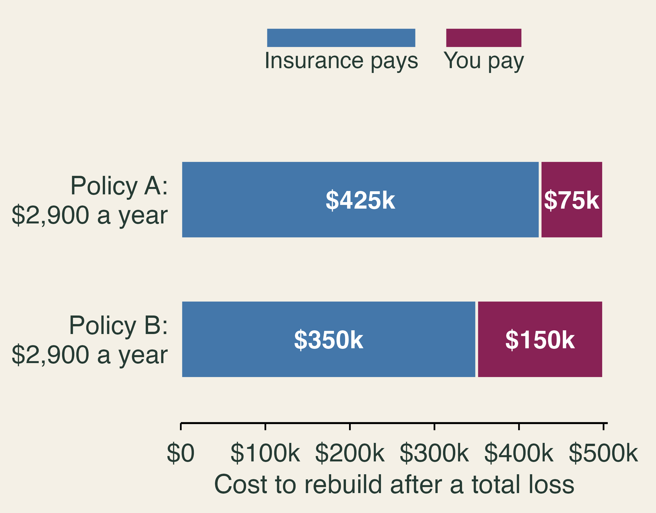
Moral hazard says insurance may lead people to take too much risk. Yet many households have the opposite problem: too little insurance. Cookson, Gallagher, and Mulder (2025) study contracts from 24 insurers in Colorado and households that lost homes in the 2021 Marshall Fire. A household is underinsured when its coverage falls short of the estimated cost of rebuilding. Among households that lost homes, a 10 percentage point increase in underinsurance reduces the probability of filing a rebuilding permit within a year by 4 percentage points. Their demand model suggests why: buyers treat insurers that write less coverage as if those insurers had lower prices. The authors call this coverage neglect, and removing it would raise consumer surplus by $290 a year, or 10% of premiums. A permit is a step toward rebuilding rather than a finished home, but it is a good early signal.

Two policies with the same premium can leave very different gaps after a total loss. Classroom numbers.

Why people underprepare

Meyer and Kunreuther (2017) organize the reasons into six biases. Myopia puts weight on today’s cost over a future benefit. Optimism says it will not happen to me. Inertia keeps the status quo. Amnesia fades the memory of past disasters. Simplification reduces risk to a label such as “not in the red zone.” Herding follows the neighbors. Some of these leave traces in market data. On amnesia, McCoy and Walsh (2018) study housing markets near severe fires in Colorado’s Front Range and conclude that fires lead to significant but short-lived increases in perceived risk. Kahn (pp. 44–45) adds a twist: after a vivid disaster, people may overestimate risk for a time, which can help if it prompts precautions.

Kahn disagrees with much of the behavioral framing. He argues that if people know there is no safety net (“no Santa Claus”), they will research their risks, and that behavioral claims can justify subsidies that favor organized interests (pp. 86–87). The two views predict different things. If people make mistakes, better prices will do little without better information or defaults. If people respond to rules, removing bailouts should change behavior. Kahn himself proposes randomized tests of insurance reforms (pp. 123–124), and that is the right way to settle the question.

Disclosure and home prices

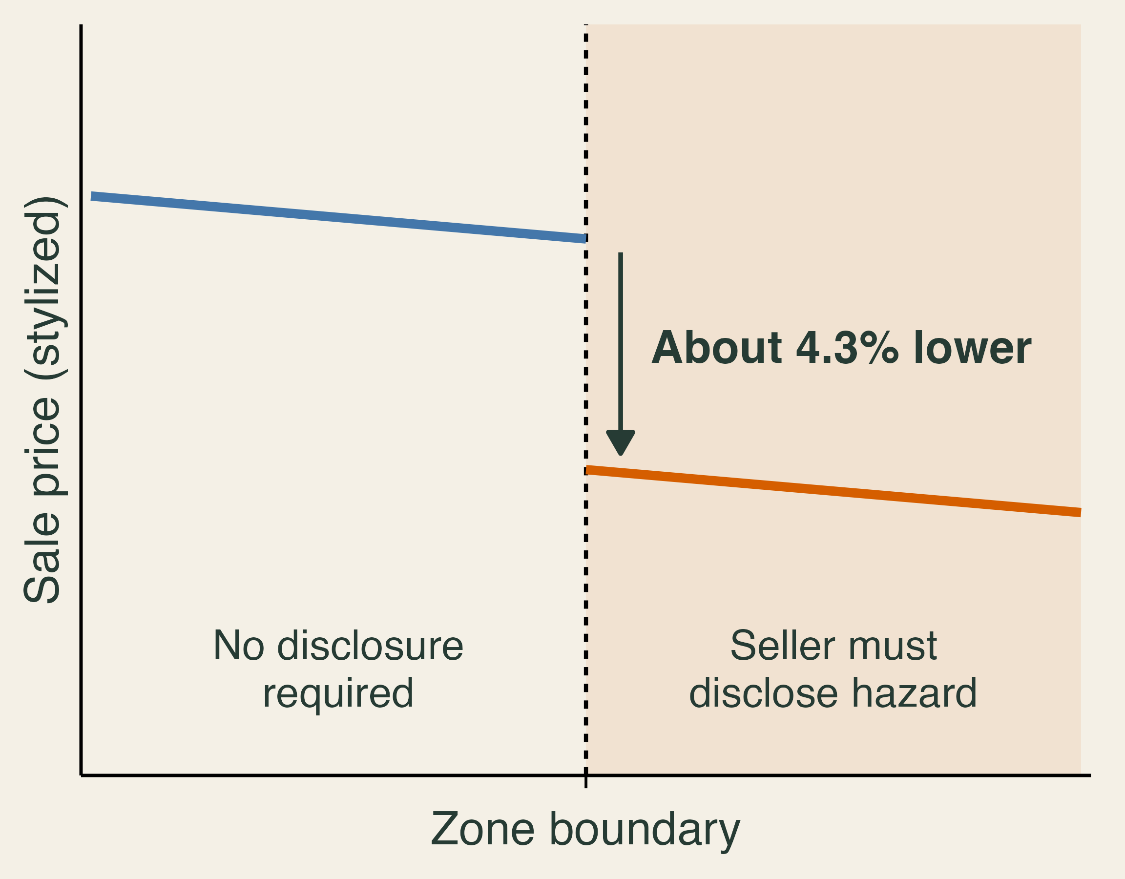
Information is the natural remedy for simplification, and disclosure laws test it. Ma et al. (2024) compare home sales near the boundaries of California’s wildfire hazard disclosure zones from 2015 to 2022. Homes required to disclose sold for about 4.3% less than nearby homes that were not, and the gap grew after damaging fires. Their boundary discontinuity design assumes that other determinants of price change smoothly at the boundary, so a jump in price at the line reflects the disclosure. This is the hedonic method from Lecture 7. The discount bundles beliefs about fire, insurance costs, and inconvenience, so it is not a fire probability. In related work, Fairweather et al. (2024) randomly showed flood-risk information to 17.5 million Redfin users and found changes in search, bidding, and purchases.

Prices step down where sellers must disclose wildfire hazard. Stylized figure based on Ma et al. (2024).

Who recovers?

Kahn (Ch. 4) divides resilience into before, during, and after a disaster, and he distinguishes between helping people and helping places (p. 40). Who recovers depends on what we measure. Baylis et al. (2026) link property damage from over 100 U.S. wildfires to tax and Census records. Residents of burned areas are wealthier than average, but inside a fire’s perimeter, lower-income homes are more likely to burn. Occupants of destroyed homes lose income for three years, adding up to 26% of a year’s pre-fire income. Residents nearby whose property was not damaged show no detectable income or employment effects. Four years later, half of destroyed addresses remain unoccupied, and reoccupied addresses house people with higher incomes than before. A street can recover while its former residents do not. The same households that cannot afford to defend against smoke (Section 2) are the least able to rebuild, so environmental justice runs through every stage of a disaster.

Why are wildfire losses rising?

We can now return to the opening question. Hazard has grown, as fires have become drier and faster. Exposure has grown, as homes have spread into the interface, helped along by free firefighting and premiums that have not always carried the risk. Smoke has stretched exposure from a burn perimeter to half a continent, so that a fire season in Quebec raises asthma visits in New York. Vulnerability persists because older homes are costly to retrofit, hardening is often not rewarded, and many households carry too little coverage or cannot afford to defend against smoke. Rising losses reflect climate, development, and institutions together.

Three limits deserve emphasis. Much of the insurance evidence comes from California, whose regulation is unusual, and several studies are working papers. The evidence on what households do is stronger than the evidence on what those actions finally save. Smoke’s damages are the hardest to see, because no one files a claim for a lost workday or a child’s asthma attack, so they depend on statistical methods and on valuation choices such as the VSL.

The most useful open question may be this one: does pricing wildfire risk reduce losses, or does it mostly move them onto other households? Insurance can get money to a family after a fire, and hardening can keep the fire from taking the house. Neither one does the other’s job, and neither one cleans the air downwind. A good policy needs all three tools: prevention, risk sharing, and cooperation across borders.

Check your understanding

1. In 2025, U.S. acres burned fell 43% from 2024 while the number of fires rose 20%. Which measure tells us more about damage, and what else would you want to know?
2. On June 7, 2023, the average monitor in the New York metro area read 153 µg/m³. Explain why this smoke is an externality, and why the Clean Air Act does little about it.
3. Zhang et al. (2025) attribute about 4,100 U.S. deaths to short-term exposure to the 2023 Canadian smoke. With a VSL of $14.2 million, what is the mortality damage? A household spent $250 on a purifier and masks during the smoke. What does that reveal about its willingness to pay to avoid smoke?
4. A $10,000 retrofit avoids $2,000 a year of expected damage to the owner’s home and $500 a year to neighbors, for five years, at a 4% discount rate. Is it worth doing for the owner? For society?
5. A household’s wealth is a $400,000 house with a 2% annual chance of total loss, and U(W) = \sqrt{W}. What is the most it would pay for full coverage? Why is the answer above $8,000?
6. Two insurers each cover 100 homes with a 2% chance of a $175,000 claim. One portfolio has independent fires; in the other, one fire reaches all 100 homes. Compare expected claims and the worst year.
7. Half of a town’s homes expect $1,000 a year in claims and half expect $5,000. What happens if insurers must charge everyone $3,000 and lower-risk owners can leave?
8. Name one wildfire policy that reduces physical losses, one that only moves them, and one that addresses smoke. Why might a town want all three?

TipCheck your answers

1. Neither is enough. Both track activity, and 2025 shows that acres can fall in a year of record damage. We would want to know where the fires burned, how intense they were, what they reached, how vulnerable it was, and where the smoke went.
2. An unpriced cost that crossed a border. New Yorkers bore health, work, and defensive costs from fires in Canada, had no say in Canadian fire management, and received no compensation; no price linked the two sides. The Clean Air Act controls domestic sources through permits and standards. A forest fire has no permit, and the Exceptional Events Rule lets states set aside smoke-affected data when EPA judges whether an area meets the standards.
3. About $58 billion, and at least $250. The damage is 4{,}100 \times \$14.2 million \approx \$58 billion. Defensive spending is a lower bound on willingness to pay: the household valued protection at no less than $250, and the purifier did not remove all of the harm. A household that could not afford a purifier would show $0 in the data despite suffering more.
4. Not for the owner, yes for society. The five-year annuity factor at 4% is 4.452. The owner’s benefit is worth $8,904, a net loss of $1,096. Adding neighbors raises the benefit to $11,130, a net gain of $1,130. A grant of at least $1,096 would change the owner’s choice.
5. About $15,840. Expected utility is 0.98 \times \sqrt{400{,}000} \approx 619.8, so the certainty equivalent is 619.8^2 \approx \$384{,}160 and the maximum premium is \$400{,}000 - \$384{,}160. It exceeds the $8,000 expected loss because of risk aversion: the household values removing the ruinous year, and the $7,840 difference is the risk premium.
6. Same average, different extremes. Expected claims are $350,000 in both. With independent fires, all 100 claiming in one year is extremely unlikely. In the correlated case, there is a 2% chance of paying $17.5 million at once.
7. The pool unravels. Lower-risk owners pay $3,000 for $1,000 of expected protection, so many leave. The remaining homes expect $5,000 each, so the break-even price rises to $5,000. This is adverse selection.
8. Answers vary. Hardening or fuel treatment reduces physical loss; insurance moves the financial loss; clean-air shelters, purifier programs, or cross-border fire cooperation address smoke. Insurance can pay for damage no one prevented, hardening can protect lives, neighbors, and uninsured values, and neither one helps the people downwind.

Textbook connection

This reading goes with Tietenberg and Lewis, Natural Resource Economics: The Essentials, 2nd edition, Chapter 12, Climate Change: Adaptation: Floods, Wildfires, and Water Scarcity, which treats wildfire as one of the adaptation challenges a warming climate brings. It also draws on Kahn, An Introduction to Natural Disaster Economics (June 2026 manuscript), for the ideas of endogenous disaster losses, risk, resilience, and insurance; page numbers appear in each section. Section 2 on smoke goes beyond both books and relies on the research cited below.

References

• Abatzoglou, J. T., and A. P. Williams (2016). Impact of anthropogenic climate change on wildfire across western US forests. Proceedings of the National Academy of Sciences 113(42), 11770–11775. doi
• Balch, J. K., et al. (2024). The fastest-growing and most destructive fires in the US (2001 to 2020). Science 386(6720), 425–431. doi
• Baylis, P., and J. Boomhower (2023). The economic incidence of wildfire suppression in the United States. American Economic Journal: Applied Economics 15(1), 442–473. doi
• Baylis, P., and J. Boomhower (2026). Mandated versus voluntary adaptation to natural disasters: The case of US wildfires. Journal of Political Economy 134(3), 895–948. doi
• Baylis, P., J. Boomhower, J. Colmer, and J. Voorheis (2026). The distribution and consequences of natural disasters: Evidence from U.S. wildfire victims. Census Bureau CES Working Paper 26-53. link
• Boomhower, J., M. Fowlie, J. Gellman, and A. Plantinga (2024, revised 2025). How are insurance markets adapting to climate change? Risk classification and pricing in the market for homeowners insurance. NBER Working Paper 32625. link
• Borgschulte, M., D. Molitor, and E. Y. Zou (2022). Air pollution and the labor market: Evidence from wildfire smoke. NBER Working Paper 29952. link
• Borgschulte, M., D. Molitor, and E. Y. Zou (2024). Air pollution and the labor market: Evidence from wildfire smoke. Review of Economics and Statistics 106(6), 1558–1575. doi
• Burke, M., et al. (2022). Exposures and behavioural responses to wildfire smoke. Nature Human Behaviour 6(10), 1351–1361. doi
• Burke, M., et al. (2023). The contribution of wildfire to PM_2.5 trends in the USA. Nature 622, 761–766. doi
• Canadian Interagency Forest Fire Centre (2024). Canada report 2023. link
• CAL FIRE (2025). Top 20 most destructive California wildfires, April 3, 2025. statistics page
• California Department of Insurance (2025). News release on the FAIR Plan assessment, February 11, 2025. link
• California FAIR Plan (2026). Key statistics and data. link
• Chen, K., Y. Ma, M. L. Bell, and W. Yang (2023). Canadian wildfire smoke and asthma syndrome emergency department visits in New York City. JAMA 330(14), 1385–1387. doi
• Cookson, J. A., E. A. Gallagher, and P. Mulder (2025). Coverage neglect in homeowners insurance. Federal Reserve Bank of Philadelphia Working Paper 25-09. doi
• Environment and Climate Change Canada and U.S. Environmental Protection Agency (2024). Review and assessment of the Canada–United States Air Quality Agreement. link
• Fairweather, D., M. E. Kahn, R. D. Metcalfe, and S. Sandoval Olascoaga (2024). Expecting climate change: A nationwide field experiment in the housing market. NBER Working Paper 33119. doi
• Government of Ontario (2019). Wildland fire management strategy. link
• Iglesias, V., J. K. Balch, and W. R. Travis (2022). U.S. fires became larger, more frequent, and more widespread in the 2000s. Science Advances 8(11), eabc0020. doi
• Jain, P., et al. (2024). Drivers and impacts of the record-breaking 2023 wildfire season in Canada. Nature Communications 15, 6764. doi
• Joo, T., M. J. Rogers, C. Soong, et al. (2024). Aged and obscured wildfire smoke associated with downwind health risks. Environmental Science & Technology Letters 11(12), 1340. doi
• Kahn, M. E. (2026). An Introduction to Natural Disaster Economics. Manuscript, June 2026.
• Keys, B. J., and P. Mulder (2024). Property insurance and disaster risk: New evidence from mortgage escrow data. NBER Working Paper 32579. doi
• Ma, L., M. Walls, M. Wibbenmeyer, and C. Lennon (2024). Risk disclosure and home prices: Evidence from California wildfire hazard zones. Land Economics 100(1), 6–21. doi
• McArdle, C. E., et al. (2023). Asthma-associated emergency department visits during the Canadian wildfire smoke episodes — United States, April–August 2023. Morbidity and Mortality Weekly Report 72(34), 926–932. doi
• McCoy, S. J., and R. P. Walsh (2018). Wildfire risk, salience & housing demand. Journal of Environmental Economics and Management 91, 203–228. doi
• Meek, H. C., et al. (2023). Notes from the field: Asthma-associated emergency department visits during a wildfire smoke event — New York, June 2023. Morbidity and Mortality Weekly Report 72(34), 933–935. doi
• Meyer, R., and H. Kunreuther (2017). The Ostrich Paradox: Why We Underprepare for Disasters. Wharton Digital Press.
• National Forestry Database. Forest fires: Area burned by cause class, 1990–2025. Canadian Council of Forest Ministers. link
• National Interagency Fire Center. Wildfires and acres; Suppression costs. link
• Natural Resources Canada (2024). The State of Canada’s Forests: Annual Report 2024. link
• New York City Public Advocate (2023). Orange sky, red alert: A review of air quality emergencies in NYC, July 11, 2023. link
• Nguyen, N., E. Macomber, M. Mastrandrea, and M. Wara (2026). The evolution of the California homeowners insurance market in the face of growing wildfire risk. Stanford Climate and Energy Policy Program. doi
• Qiu, M., et al. (2025). Wildfire smoke exposure and mortality burden in the USA under climate change. Nature 647, 935–943. doi
• Radeloff, V. C., et al. (2018). Rapid growth of the US wildland-urban interface raises wildfire risk. Proceedings of the National Academy of Sciences 115(13), 3314–3319. doi
• SOPFEU, Société de protection des forêts contre le feu (2026). Current situation: Northern zone. link
• Schollaert, C. L., et al. (2024). Quantifying the smoke-related public health trade-offs of forest management. Nature Sustainability 7, 130–139. doi
• Tietenberg, T., and L. Lewis (2025). Natural Resource Economics: The Essentials, 2nd edition. Routledge.
• U.S. Department of Transportation (2026). Departmental guidance on valuation of a statistical life in economic analysis, revised March 2026. link
• U.S. Environmental Protection Agency (2016). Treatment of data influenced by exceptional events; final rule. Federal Register 81, 68216–68282, October 3, 2016. link
• U.S. Environmental Protection Agency (2026). Mortality risk valuation. link
• U.S. Environmental Protection Agency. Air Quality System pre-generated data files: daily PM_2.5 (daily_88101_2023) and daily AQI by core-based statistical area, 2000–2025. link
• U.S. Forest Service (2022). National Prescribed Fire Program Review. link
• Wallace, N. (2026). A review and evaluation of the California FAIR Plan. Working paper, Haas School of Business, UC Berkeley. link
• Zhang, Q., et al. (2025). Long-range PM_2.5 pollution and health impacts from the 2023 Canadian wildfires. Nature 645, 672–678. doi